CS231N

This course is a deep dive into the details of deep learning architectures with a focus on learning end-to-end models for these tasks, particularly image classification

This page contains my solutions and approaches for the assignment All source codes of my solutions are available on GitHub

Softmax exercise

Complete and hand in this completed worksheet (including its outputs and any supporting code outside of the worksheet) with your assignment submission. For more details see the assignments page on the course website.

This exercise is analogous to the SVM exercise. You will:

implement a fully-vectorized loss function for the Softmax classifier
implement the fully-vectorized expression for its analytic gradient
check your implementation with numerical gradient
use a validation set to tune the learning rate and regularization strength
optimize the loss function with SGD
visualize the final learned weights

Import necessary packages

import random
import numpy as np
from cs231n.data_utils import load_CIFAR10
import matplotlib.pyplot as plt

%matplotlib inline
plt.rcParams['figure.figsize'] = (10.0, 8.0) # set default size of plots
plt.rcParams['image.interpolation'] = 'nearest'
plt.rcParams['image.cmap'] = 'gray'

# for auto-reloading extenrnal modules
# see http://stackoverflow.com/questions/1907993/autoreload-of-modules-in-ipython
%load_ext autoreload
%autoreload 2

CIFAR-10 Data Loading and Preprocessing

def get_CIFAR10_data(num_training=49000, num_validation=1000, num_test=1000, num_dev=500):
    """
    Load the CIFAR-10 dataset from disk and perform preprocessing to prepare
    it for the linear classifier. These are the same steps as we used for the
    SVM, but condensed to a single function.  
    """
    # Load the raw CIFAR-10 data
    cifar10_dir = 'cs231n/datasets/cifar-10-batches-py'
    
    # Cleaning up variables to prevent loading data multiple times (which may cause memory issue)
    try:
       del X_train, y_train
       del X_test, y_test
       print('Clear previously loaded data.')
    except:
       pass

    X_train, y_train, X_test, y_test = load_CIFAR10(cifar10_dir)
    
    # subsample the data
    mask = list(range(num_training, num_training + num_validation))
    X_val = X_train[mask]
    y_val = y_train[mask]
    mask = list(range(num_training))
    X_train = X_train[mask]
    y_train = y_train[mask]
    mask = list(range(num_test))
    X_test = X_test[mask]
    y_test = y_test[mask]
    mask = np.random.choice(num_training, num_dev, replace=False)
    X_dev = X_train[mask]
    y_dev = y_train[mask]
    
    # Preprocessing: reshape the image data into rows
    X_train = np.reshape(X_train, (X_train.shape[0], -1))
    X_val = np.reshape(X_val, (X_val.shape[0], -1))
    X_test = np.reshape(X_test, (X_test.shape[0], -1))
    X_dev = np.reshape(X_dev, (X_dev.shape[0], -1))
    
    # Normalize the data: subtract the mean image
    mean_image = np.mean(X_train, axis = 0)
    X_train -= mean_image
    X_val -= mean_image
    X_test -= mean_image
    X_dev -= mean_image
    
    # add bias dimension and transform into columns
    X_train = np.hstack([X_train, np.ones((X_train.shape[0], 1))])
    X_val = np.hstack([X_val, np.ones((X_val.shape[0], 1))])
    X_test = np.hstack([X_test, np.ones((X_test.shape[0], 1))])
    X_dev = np.hstack([X_dev, np.ones((X_dev.shape[0], 1))])
    
    return X_train, y_train, X_val, y_val, X_test, y_test, X_dev, y_dev


# Invoke the above function to get our data.
X_train, y_train, X_val, y_val, X_test, y_test, X_dev, y_dev = get_CIFAR10_data()
print('Train data shape: ', X_train.shape)
print('Train labels shape: ', y_train.shape)
print('Validation data shape: ', X_val.shape)
print('Validation labels shape: ', y_val.shape)
print('Test data shape: ', X_test.shape)
print('Test labels shape: ', y_test.shape)
print('dev data shape: ', X_dev.shape)
print('dev labels shape: ', y_dev.shape)

Train data shape:  (49000, 3073)
Train labels shape:  (49000,)
Validation data shape:  (1000, 3073)
Validation labels shape:  (1000,)
Test data shape:  (1000, 3073)
Test labels shape:  (1000,)
dev data shape:  (500, 3073)
dev labels shape:  (500,)

Softmax Classifier

Your code for this section will all be written inside cs231n/classifiers/softmax.py.

# First implement the naive softmax loss function with nested loops.
# Open the file cs231n/classifiers/softmax.py and implement the
# softmax_loss_naive function.

from cs231n.classifiers.softmax import softmax_loss_naive
import time

# Generate a random softmax weight matrix and use it to compute the loss.
W = np.random.randn(3073, 10) * 0.0001
loss, grad = softmax_loss_naive(W, X_dev, y_dev, 0.0)

# As a rough sanity check, our loss should be something close to -log(0.1).
print('loss: %f' % loss)
print('sanity check: %f' % (-np.log(0.1)))

loss: 2.367588
sanity check: 2.302585

softmax_loss_naive

def softmax_loss_naive(W, X, y, reg):
    """
    Softmax loss function, naive implementation (with loops)

    Inputs have dimension D, there are C classes, and we operate on minibatches
    of N examples.

    Inputs:
    - W: A numpy array of shape (D, C) containing weights.
    - X: A numpy array of shape (N, D) containing a minibatch of data.
    - y: A numpy array of shape (N,) containing training labels; y[i] = c means
      that X[i] has label c, where 0 <= c < C.
    - reg: (float) regularization strength

    Returns a tuple of:
    - loss as single float
    - gradient with respect to weights W; an array of same shape as W
    """
    # Initialize the loss and gradient to zero.
    loss = 0.0
    dW = np.zeros_like(W)
    N = X.shape[0]
    C = W.shape[1]
    #############################################################################
    # TODO: Compute the softmax loss and its gradient using explicit loops.     #
    # Store the loss in loss and the gradient in dW. If you are not careful     #
    # here, it is easy to run into numeric instability. Don't forget the        #
    # regularization!                                                           #
    #############################################################################
    # *****START OF YOUR CODE (DO NOT DELETE/MODIFY THIS LINE)*****

    for i in range(N):
      scores = X[i].dot(W)
      scores = scores - max(scores) #for numerical stability http://saitcelebi.com/tut/output/part2.html
      exps = np.exp(scores)
      sum_of_exps = np.sum(exps)
      normalized_probs = exps / sum_of_exps
      correct_class_prob = normalized_probs[y[i]]
      curent_loss = - np.log(correct_class_prob)
      loss += curent_loss

      for j in range(C):
        if j == y[i]:
          dW[:, j] += X[i] * (normalized_probs[j] + -1)
        else:
          dW[:, j] += X[i] * normalized_probs[j]
      
        
        

    loss /= N
    dW /= N

    loss += reg * np.sum(W * W)
    dW += 2 * reg * W

    # *****END OF YOUR CODE (DO NOT DELETE/MODIFY THIS LINE)*****

    return loss, dW

Inline Question 1

Why do we expect our loss to be close to -log(0.1)? Explain briefly.**

\(\color{blue}{\textit Your Answer:}\) Fill this in

# Complete the implementation of softmax_loss_naive and implement a (naive)
# version of the gradient that uses nested loops.
loss, grad = softmax_loss_naive(W, X_dev, y_dev, 0.0)

# As we did for the SVM, use numeric gradient checking as a debugging tool.
# The numeric gradient should be close to the analytic gradient.
from cs231n.gradient_check import grad_check_sparse
f = lambda w: softmax_loss_naive(w, X_dev, y_dev, 0.0)[0]
grad_numerical = grad_check_sparse(f, W, grad, 10)

# similar to SVM case, do another gradient check with regularization
loss, grad = softmax_loss_naive(W, X_dev, y_dev, 5e1)
f = lambda w: softmax_loss_naive(w, X_dev, y_dev, 5e1)[0]
grad_numerical = grad_check_sparse(f, W, grad, 10)

numerical: 1.851181 analytic: 1.851181, relative error: 1.190161e-08
numerical: -1.589167 analytic: -1.589167, relative error: 1.965947e-08
numerical: -1.745848 analytic: -1.745849, relative error: 4.023629e-08
numerical: -1.976393 analytic: -1.976393, relative error: 1.687936e-09
numerical: -2.633638 analytic: -2.633638, relative error: 4.019499e-09
numerical: -0.051344 analytic: -0.051344, relative error: 9.577136e-07
numerical: 0.694378 analytic: 0.694378, relative error: 1.298612e-07
numerical: -0.086835 analytic: -0.086835, relative error: 1.495133e-07
numerical: 0.940912 analytic: 0.940912, relative error: 4.646779e-08
numerical: 0.609976 analytic: 0.609976, relative error: 1.151788e-08
numerical: -0.675575 analytic: -0.675575, relative error: 6.531062e-09
numerical: 0.456932 analytic: 0.456932, relative error: 1.137939e-09
numerical: -1.450736 analytic: -1.450736, relative error: 1.654804e-08
numerical: 1.836381 analytic: 1.836381, relative error: 1.943110e-08
numerical: 1.318572 analytic: 1.318572, relative error: 5.475544e-08
numerical: 0.631718 analytic: 0.631718, relative error: 2.148730e-09
numerical: -2.560153 analytic: -2.560154, relative error: 1.407254e-08
numerical: 3.494902 analytic: 3.494902, relative error: 2.979533e-08
numerical: 0.622316 analytic: 0.622316, relative error: 6.834693e-08
numerical: 1.001572 analytic: 1.001572, relative error: 5.033441e-08

softmax_loss_vectorized

def softmax_loss_vectorized(W, X, y, reg):
    """
    Softmax loss function, vectorized version.

    Inputs and outputs are the same as softmax_loss_naive.
    """
    # Initialize the loss and gradient to zero.
    loss = 0.0
    dW = np.zeros_like(W)

    N = X.shape[0]
    C = W.shape[1]
    #############################################################################
    # TODO: Compute the softmax loss and its gradient using no explicit loops.  #
    # Store the loss in loss and the gradient in dW. If you are not careful     #
    # here, it is easy to run into numeric instability. Don't forget the        #
    # regularization!                                                           #
    #############################################################################
    # *****START OF YOUR CODE (DO NOT DELETE/MODIFY THIS LINE)*****

    scores = X.dot(W)
    scores = scores - np.max(scores, axis=-1, keepdims=True) # numerical stabilization
    exps = np.exp(scores)
    probs = exps / np.sum(exps, axis=-1, keepdims=True)
    correct_class_probs = probs[np.arange(len(probs)), y]
    loss =  - np.sum(np.log(correct_class_probs))
    
    probs_for_gradient = probs
    probs_for_gradient[np.arange(len(probs)), y] -= 1

    dW += np.dot(X.T, probs_for_gradient)

    # *****END OF YOUR CODE (DO NOT DELETE/MODIFY THIS LINE)*****

    loss /= N
    dW /= N

    loss += reg * np.sum(W * W)
    dW += 2 * reg * W


    return loss, dW

# Now that we have a naive implementation of the softmax loss function and its gradient,
# implement a vectorized version in softmax_loss_vectorized.
# The two versions should compute the same results, but the vectorized version should be
# much faster.
tic = time.time()
loss_naive, grad_naive = softmax_loss_naive(W, X_dev, y_dev, 0.000005)
toc = time.time()
print('naive loss: %e computed in %fs' % (loss_naive, toc - tic))

from cs231n.classifiers.softmax import softmax_loss_vectorized
tic = time.time()
loss_vectorized, grad_vectorized = softmax_loss_vectorized(W, X_dev, y_dev, 0.000005)
toc = time.time()
print('vectorized loss: %e computed in %fs' % (loss_vectorized, toc - tic))

# As we did for the SVM, we use the Frobenius norm to compare the two versions
# of the gradient.
grad_difference = np.linalg.norm(grad_naive - grad_vectorized, ord='fro')
print('Loss difference: %f' % np.abs(loss_naive - loss_vectorized))
print('Gradient difference: %f' % grad_difference)

naive loss: 2.367588e+00 computed in 0.124651s
vectorized loss: 2.367588e+00 computed in 0.013923s
Loss difference: 0.000000
Gradient difference: 0.000000

Time Comparison

### finding an iteration number

# In the file linear_classifier.py, implement SGD in the function
# LinearClassifier.train() and then run it with the code below.
from cs231n.classifiers import Softmax
model = Softmax()
tic = time.time()
loss_hist = model.train(X_train, y_train, learning_rate=1e-7, reg=2.5e4,
                      num_iters=1500, verbose=True)
toc = time.time()
print('That took %fs' % (toc - tic))

# A useful debugging strategy is to plot the loss as a function of
# iteration number:
plt.plot(loss_hist)
plt.xlabel('Iteration number')
plt.ylabel('Loss value')
plt.show()

iteration 0 / 1500: loss 774.598624
iteration 100 / 1500: loss 283.944292
iteration 200 / 1500: loss 105.330389
iteration 300 / 1500: loss 39.822003
iteration 400 / 1500: loss 15.941602
iteration 500 / 1500: loss 7.140703
iteration 600 / 1500: loss 3.929613
iteration 700 / 1500: loss 2.796842
iteration 800 / 1500: loss 2.368988
iteration 900 / 1500: loss 2.167978
iteration 1000 / 1500: loss 2.079389
iteration 1100 / 1500: loss 2.077780
iteration 1200 / 1500: loss 2.052574
iteration 1300 / 1500: loss 2.082320
iteration 1400 / 1500: loss 2.062715
That took 11.717951s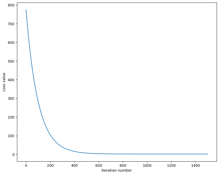

Grid Search

# Use the validation set to tune hyperparameters (regularization strength and
# learning rate). You should experiment with different ranges for the learning
# rates and regularization strengths; if you are careful you should be able to
# get a classification accuracy of over 0.35 on the validation set.

from cs231n.classifiers import Softmax
results = {}
best_val = -1
best_softmax = None

################################################################################
# TODO:                                                                        #
# Use the validation set to set the learning rate and regularization strength. #
# This should be identical to the validation that you did for the SVM; save    #
# the best trained softmax classifer in best_softmax.                          #
################################################################################

# Provided as a reference. You may or may not want to change these hyperparameters
learning_rates = [1e-7, 5e-7, 1e-6]
regularization_strengths = [1e4, 2.5e4, 5e4]

# *****START OF YOUR CODE (DO NOT DELETE/MODIFY THIS LINE)*****

import itertools
for lr, reg in itertools.product(learning_rates, regularization_strengths):
  model = Softmax()
  loss_hist = model.train(X_train, y_train, learning_rate=lr, reg=reg,
                        num_iters=1000, verbose=False)
  y_train_pred = model.predict(X_train)
  train_accuracy = np.mean(y_train == y_train_pred)
  y_val_pred = model.predict(X_val)
  val_accuracy  = np.mean(y_val == y_val_pred)
  results[(lr, reg)] = train_accuracy, val_accuracy
  if val_accuracy > best_val:
    best_val = val_accuracy
    best_softmax = model


# *****END OF YOUR CODE (DO NOT DELETE/MODIFY THIS LINE)*****
    
# Print out results.
for lr, reg in sorted(results):
    train_accuracy, val_accuracy = results[(lr, reg)]
    print('lr %e reg %e train accuracy: %f val accuracy: %f' % (
                lr, reg, train_accuracy, val_accuracy))
    
print('best validation accuracy achieved during cross-validation: %f' % best_val)

lr 1.000000e-07 reg 1.000000e+04 train accuracy: 0.328204 val accuracy: 0.347000
lr 1.000000e-07 reg 2.500000e+04 train accuracy: 0.333714 val accuracy: 0.348000
lr 1.000000e-07 reg 5.000000e+04 train accuracy: 0.306122 val accuracy: 0.325000
lr 5.000000e-07 reg 1.000000e+04 train accuracy: 0.351939 val accuracy: 0.357000
lr 5.000000e-07 reg 2.500000e+04 train accuracy: 0.327204 val accuracy: 0.336000
lr 5.000000e-07 reg 5.000000e+04 train accuracy: 0.309469 val accuracy: 0.311000
lr 1.000000e-06 reg 1.000000e+04 train accuracy: 0.348102 val accuracy: 0.365000
lr 1.000000e-06 reg 2.500000e+04 train accuracy: 0.323429 val accuracy: 0.328000
lr 1.000000e-06 reg 5.000000e+04 train accuracy: 0.289653 val accuracy: 0.301000
best validation accuracy achieved during cross-validation: 0.365000

# Visualize the cross-validation results
import math
import pdb

# pdb.set_trace()

x_scatter = [math.log10(x[0]) for x in results]
y_scatter = [math.log10(x[1]) for x in results]

# plot training accuracy
marker_size = 100
colors = [results[x][0] for x in results]
plt.subplot(2, 1, 1)
plt.tight_layout(pad=3)
plt.scatter(x_scatter, y_scatter, marker_size, c=colors, cmap=plt.cm.coolwarm)
plt.colorbar()
plt.xlabel('log learning rate')
plt.ylabel('log regularization strength')
plt.title('CIFAR-10 training accuracy')

# plot validation accuracy
colors = [results[x][1] for x in results] # default size of markers is 20
plt.subplot(2, 1, 2)
plt.scatter(x_scatter, y_scatter, marker_size, c=colors, cmap=plt.cm.coolwarm)
plt.colorbar()
plt.xlabel('log learning rate')
plt.ylabel('log regularization strength')
plt.title('CIFAR-10 validation accuracy')
plt.show()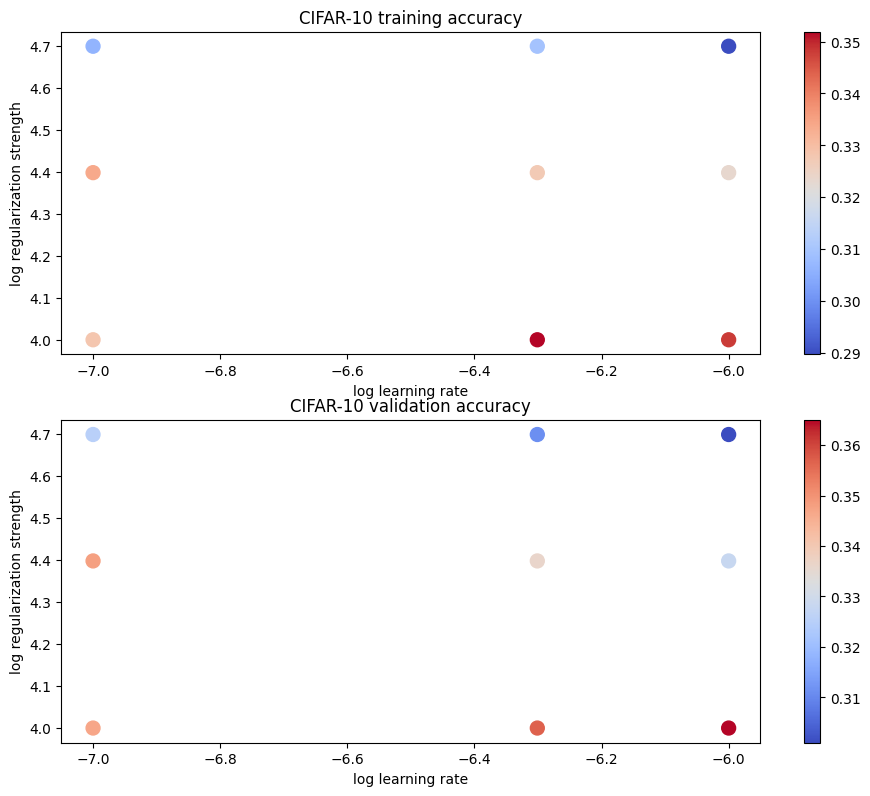

Training Best Model

# evaluate on test set
# Evaluate the best softmax on test set
y_test_pred = best_softmax.predict(X_test)
test_accuracy = np.mean(y_test == y_test_pred)
print('softmax on raw pixels final test set accuracy: %f' % (test_accuracy, ))

softmax on raw pixels final test set accuracy: 0.352000

Inline Question 2 - True or False

Suppose the overall training loss is defined as the sum of the per-datapoint loss over all training examples. It is possible to add a new datapoint to a training set that would leave the SVM loss unchanged, but this is not the case with the Softmax classifier loss.

\(\color{blue}{\textit Your Answer:}\)

\(\color{blue}{\textit Your Explanation:}\)

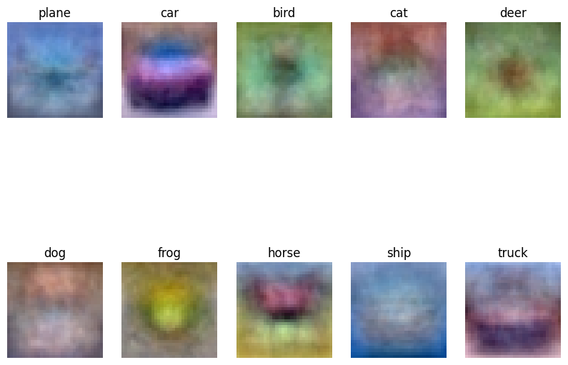
Visualizing learned weights

# Visualize the learned weights for each class
w = best_softmax.W[:-1,:] # strip out the bias
w = w.reshape(32, 32, 3, 10)

w_min, w_max = np.min(w), np.max(w)

classes = ['plane', 'car', 'bird', 'cat', 'deer', 'dog', 'frog', 'horse', 'ship', 'truck']
for i in range(10):
    plt.subplot(2, 5, i + 1)
    
    # Rescale the weights to be between 0 and 255
    wimg = 255.0 * (w[:, :, :, i].squeeze() - w_min) / (w_max - w_min)
    plt.imshow(wimg.astype('uint8'))
    plt.axis('off')
    plt.title(classes[i])