# As usual, a bit of setup
from __future__ import print_function
import time
import numpy as np
import matplotlib.pyplot as plt
from cs231n.classifiers.fc_net import *
from cs231n.data_utils import get_CIFAR10_data
from cs231n.gradient_check import eval_numerical_gradient, eval_numerical_gradient_array
from cs231n.solver import Solver
%matplotlib inline
plt.rcParams['figure.figsize'] = (10.0, 8.0) # set default size of plots
plt.rcParams['image.interpolation'] = 'nearest'
plt.rcParams['image.cmap'] = 'gray'
# for auto-reloading external modules
# see http://stackoverflow.com/questions/1907993/autoreload-of-modules-in-ipython
%load_ext autoreload
%autoreload 2
def rel_error(x, y):
""" returns relative error """
return np.max(np.abs(x - y) / (np.maximum(1e-8, np.abs(x) + np.abs(y))))CS231N
This course is a deep dive into the details of deep learning architectures with a focus on learning end-to-end models for these tasks, particularly image classification
This page contains my solutions and approaches for the assignment All source codes of my solutions are available on GitHub
Fully-Connected Neural Nets
In this exercise we will implement fully-connected networks using a modular approach. For each layer we will implement a forward and a backward function. The forward function will receive inputs, weights, and other parameters and will return both an output and a cache object storing data needed for the backward pass, like this:
def layer_forward(x, w):
  """ Receive inputs x and weights w """
  # Do some computations ...
  z = # ... some intermediate value
  # Do some more computations ...
  out = # the output

  cache = (x, w, z, out) # Values we need to compute gradients

  return out, cache
The backward pass will receive upstream derivatives and the cache object, and will return gradients with respect to the inputs and weights, like this:
def layer_backward(dout, cache):
  """
  Receive dout (derivative of loss with respect to outputs) and cache,
  and compute derivative with respect to inputs.
  """
  # Unpack cache values
  x, w, z, out = cache

  # Use values in cache to compute derivatives
  dx = # Derivative of loss with respect to x
  dw = # Derivative of loss with respect to w

  return dx, dw
After implementing a bunch of layers this way, we will be able to easily combine them to build classifiers with different architectures.
Import necessary packages
CIFAR-10 Data Loading and Preprocessing
# Load the (preprocessed) CIFAR10 data.

data = get_CIFAR10_data()
for k, v in list(data.items()):
  print(('%s: ' % k, v.shape))
('X_train: ', (49000, 3, 32, 32))
('y_train: ', (49000,))
('X_val: ', (1000, 3, 32, 32))
('y_val: ', (1000,))
('X_test: ', (1000, 3, 32, 32))
('y_test: ', (1000,))Affine layer: forward
Open the file cs231n/layers.py and implement the affine_forward function.
Once you are done you can test your implementaion by running the following:
def affine_forward(x, w, b):
    """
    Computes the forward pass for an affine (fully-connected) layer.

    The input x has shape (N, d_1, ..., d_k) and contains a minibatch of N
    examples, where each example x[i] has shape (d_1, ..., d_k). We will
    reshape each input into a vector of dimension D = d_1 * ... * d_k, and
    then transform it to an output vector of dimension M.

    Inputs:
    - x: A numpy array containing input data, of shape (N, d_1, ..., d_k)
    - w: A numpy array of weights, of shape (D, M)
    - b: A numpy array of biases, of shape (M,)

    Returns a tuple of:
    - out: output, of shape (N, M)
    - cache: (x, w, b)
    """
    out = None
    ###########################################################################
    # TODO: Implement the affine forward pass. Store the result in out. You   #
    # will need to reshape the input into rows.                               #
    ###########################################################################
    # *****START OF YOUR CODE (DO NOT DELETE/MODIFY THIS LINE)*****

    x_rows = np.reshape(x, (x.shape[0], -1))
    out = np.dot(x_rows, w) + b

    # *****END OF YOUR CODE (DO NOT DELETE/MODIFY THIS LINE)*****
    ###########################################################################
    #                             END OF YOUR CODE                            #
    ###########################################################################
    cache = (x, w, b)
    return out, cache
# Test the affine_forward function
num_inputs = 2
input_shape = (4, 5, 6)
output_dim = 3
input_size = num_inputs * np.prod(input_shape)
weight_size = output_dim * np.prod(input_shape)
x = np.linspace(-0.1, 0.5, num=input_size).reshape(num_inputs, *input_shape)
w = np.linspace(-0.2, 0.3, num=weight_size).reshape(np.prod(input_shape), output_dim)
b = np.linspace(-0.3, 0.1, num=output_dim)
out, _ = affine_forward(x, w, b)
correct_out = np.array([[ 1.49834967, 1.70660132, 1.91485297],
[ 3.25553199, 3.5141327, 3.77273342]])
# Compare your output with ours. The error should be around e-9 or less.
print('Testing affine_forward function:')
print('difference: ', rel_error(out, correct_out))Testing affine_forward function:
difference: 9.769849468192957e-10Affine layer: backward
Now implement the affine_backward function and test your implementation using numeric gradient checking.
def affine_backward(dout, cache):
    """
    Computes the backward pass for an affine layer.

    Inputs:
    - dout: Upstream derivative, of shape (N, M)
    - cache: Tuple of:
      - x: Input data, of shape (N, d_1, ... d_k)
      - w: Weights, of shape (D, M)
      - b: Biases, of shape (M,)

    Returns a tuple of:
    - dx: Gradient with respect to x, of shape (N, d1, ..., d_k)
    - dw: Gradient with respect to w, of shape (D, M)
    - db: Gradient with respect to b, of shape (M,)
    """
    x, w, b = cache
    dx, dw, db = None, None, None
    ###########################################################################
    # TODO: Implement the affine backward pass.                               #
    ###########################################################################
    # *****START OF YOUR CODE (DO NOT DELETE/MODIFY THIS LINE)*****

    x_rows = np.reshape(x, (x.shape[0], -1))

    dx = np.dot(dout, w.T)
    dx = np.reshape(dx, x.shape)
    dw = np.dot(x_rows.T, dout)
    db = np.sum(dout, axis=0)


    # *****END OF YOUR CODE (DO NOT DELETE/MODIFY THIS LINE)*****
    ###########################################################################
    #                             END OF YOUR CODE                            #
    ###########################################################################
    return dx, dw, db
# Test the affine_backward function
np.random.seed(231)
x = np.random.randn(10, 2, 3)
w = np.random.randn(6, 5)
b = np.random.randn(5)
dout = np.random.randn(10, 5)
dx_num = eval_numerical_gradient_array(lambda x: affine_forward(x, w, b)[0], x, dout)
dw_num = eval_numerical_gradient_array(lambda w: affine_forward(x, w, b)[0], w, dout)
db_num = eval_numerical_gradient_array(lambda b: affine_forward(x, w, b)[0], b, dout)
_, cache = affine_forward(x, w, b)
dx, dw, db = affine_backward(dout, cache)
# The error should be around e-10 or less
print('Testing affine_backward function:')
print('dx error: ', rel_error(dx_num, dx))
print('dw error: ', rel_error(dw_num, dw))
print('db error: ', rel_error(db_num, db))Testing affine_backward function:
dx error: 5.399100368651805e-11
dw error: 9.904211865398145e-11
db error: 2.4122867568119087e-11ReLU activation: forward
Implement the forward pass for the ReLU activation function in the relu_forward function and test your implementation using the following:
def relu_forward(x):
    """
    Computes the forward pass for a layer of rectified linear units (ReLUs).

    Input:
    - x: Inputs, of any shape

    Returns a tuple of:
    - out: Output, of the same shape as x
    - cache: x
    """
    out = None
    ###########################################################################
    # TODO: Implement the ReLU forward pass.                                  #
    ###########################################################################
    # *****START OF YOUR CODE (DO NOT DELETE/MODIFY THIS LINE)*****

    out = np.maximum(0.0, x)

    # *****END OF YOUR CODE (DO NOT DELETE/MODIFY THIS LINE)*****
    ###########################################################################
    #                             END OF YOUR CODE                            #
    ###########################################################################
    cache = x
    return out, cache
# Test the relu_forward function
x = np.linspace(-0.5, 0.5, num=12).reshape(3, 4)
out, _ = relu_forward(x)
correct_out = np.array([[ 0., 0., 0., 0., ],
[ 0., 0., 0.04545455, 0.13636364,],
[ 0.22727273, 0.31818182, 0.40909091, 0.5, ]])
# Compare your output with ours. The error should be on the order of e-8
print('Testing relu_forward function:')
print('difference: ', rel_error(out, correct_out))Testing relu_forward function:
difference: 4.999999798022158e-08ReLU activation: backward
Now implement the backward pass for the ReLU activation function in the relu_backward function and test your implementation using numeric gradient checking:
def relu_backward(dout, cache):
    """
    Computes the backward pass for a layer of rectified linear units (ReLUs).

    Input:
    - dout: Upstream derivatives, of any shape
    - cache: Input x, of same shape as dout

    Returns:
    - dx: Gradient with respect to x
    """
    dx, x = None, cache
    ###########################################################################
    # TODO: Implement the ReLU backward pass.                                 #
    ###########################################################################
    # *****START OF YOUR CODE (DO NOT DELETE/MODIFY THIS LINE)*****

    dx = (x>0).astype(x.dtype) * dout

    # *****END OF YOUR CODE (DO NOT DELETE/MODIFY THIS LINE)*****
    ###########################################################################
    #                             END OF YOUR CODE                            #
    ###########################################################################
return dxnp.random.seed(231)
x = np.random.randn(10, 10)
dout = np.random.randn(*x.shape)
dx_num = eval_numerical_gradient_array(lambda x: relu_forward(x)[0], x, dout)
_, cache = relu_forward(x)
dx = relu_backward(dout, cache)
# The error should be on the order of e-12
print('Testing relu_backward function:')
print('dx error: ', rel_error(dx_num, dx))Testing relu_backward function:
dx error: 3.2756349136310288e-12Inline Question 1:
We’ve only asked you to implement ReLU, but there are a number of different activation functions that one could use in neural networks, each with its pros and cons. In particular, an issue commonly seen with activation functions is getting zero (or close to zero) gradient flow during backpropagation. Which of the following activation functions have this problem? If you consider these functions in the one dimensional case, what types of input would lead to this behaviour? 1. Sigmoid 2. ReLU 3. Leaky ReLU
Answer:
[FILL THIS IN]
“Sandwich” layers
There are some common patterns of layers that are frequently used in neural nets. For example, affine layers are frequently followed by a ReLU nonlinearity. To make these common patterns easy, we define several convenience layers in the file cs231n/layer_utils.py.
For now take a look at the affine_relu_forward and affine_relu_backward functions, and run the following to numerically gradient check the backward pass:
def affine_relu_forward(x, w, b):
    """
    Convenience layer that perorms an affine transform followed by a ReLU

    Inputs:
    - x: Input to the affine layer
    - w, b: Weights for the affine layer

    Returns a tuple of:
    - out: Output from the ReLU
    - cache: Object to give to the backward pass
    """
    a, fc_cache = affine_forward(x, w, b)
    out, relu_cache = relu_forward(a)
    cache = (fc_cache, relu_cache)
    return out, cache


def affine_relu_backward(dout, cache):
    """
    Backward pass for the affine-relu convenience layer
    """
    fc_cache, relu_cache = cache
    da = relu_backward(dout, relu_cache)
    dx, dw, db = affine_backward(da, fc_cache)
    return dx, dw, db
from cs231n.layer_utils import affine_relu_forward, affine_relu_backward
np.random.seed(231)
x = np.random.randn(2, 3, 4)
w = np.random.randn(12, 10)
b = np.random.randn(10)
dout = np.random.randn(2, 10)
out, cache = affine_relu_forward(x, w, b)
dx, dw, db = affine_relu_backward(dout, cache)
dx_num = eval_numerical_gradient_array(lambda x: affine_relu_forward(x, w, b)[0], x, dout)
dw_num = eval_numerical_gradient_array(lambda w: affine_relu_forward(x, w, b)[0], w, dout)
db_num = eval_numerical_gradient_array(lambda b: affine_relu_forward(x, w, b)[0], b, dout)
# Relative error should be around e-10 or less
print('Testing affine_relu_forward and affine_relu_backward:')
print('dx error: ', rel_error(dx_num, dx))
print('dw error: ', rel_error(dw_num, dw))
print('db error: ', rel_error(db_num, db))Testing affine_relu_forward and affine_relu_backward:
dx error: 2.299579177309368e-11
dw error: 8.162011105764925e-11
db error: 7.826724021458994e-12Loss layers: Softmax and SVM
Now implement the loss and gradient for softmax and SVM in the softmax_loss and svm_loss function in cs231n/layers.py. These should be similar to what you implemented in cs231n/classifiers/softmax.py and cs231n/classifiers/linear_svm.py.
You can make sure that the implementations are correct by running the following:
def softmax_loss(x, y):
    """
    Computes the loss and gradient for softmax classification.

    Inputs:
    - x: Input data, of shape (N, C) where x[i, j] is the score for the jth
      class for the ith input.
    - y: Vector of labels, of shape (N,) where y[i] is the label for x[i] and
      0 <= y[i] < C

    Returns a tuple of:
    - loss: Scalar giving the loss
    - dx: Gradient of the loss with respect to x
    """
    loss, dx = None, None

    ###########################################################################
    # TODO: Copy over your solution from A1.
    ###########################################################################
    # *****START OF YOUR CODE (DO NOT DELETE/MODIFY THIS LINE)*****
    N = x.shape[0]
    exps = np.exp(x)
    probs = exps / np.sum(exps, axis=-1, keepdims=True)
    correct_class_probs = probs[np.arange(len(probs)), y]
    loss =  - np.sum(np.log(correct_class_probs))

    dx = probs
    dx[np.arange(len(probs)), y] -= 1

    loss /= N
    dx /= N

    # *****END OF YOUR CODE (DO NOT DELETE/MODIFY THIS LINE)*****
    ###########################################################################
    #                             END OF YOUR CODE                            #
    ###########################################################################
return loss, dxnp.random.seed(231)
num_classes, num_inputs = 10, 50
x = 0.001 * np.random.randn(num_inputs, num_classes)
y = np.random.randint(num_classes, size=num_inputs)
dx_num = eval_numerical_gradient(lambda x: svm_loss(x, y)[0], x, verbose=False)
loss, dx = svm_loss(x, y)
# Test svm_loss function. Loss should be around 9 and dx error should be around the order of e-9
print('Testing svm_loss:')
print('loss: ', loss)
print('dx error: ', rel_error(dx_num, dx))
dx_num = eval_numerical_gradient(lambda x: softmax_loss(x, y)[0], x, verbose=False)
loss, dx = softmax_loss(x, y)
# Test softmax_loss function. Loss should be close to 2.3 and dx error should be around e-8
print('\nTesting softmax_loss:')
print('loss: ', loss)
print('dx error: ', rel_error(dx_num, dx))Testing svm_loss:
loss: 8.999602749096233
dx error: 1.4021566006651672e-09
Testing softmax_loss:
loss: 2.302545844500738
dx error: 9.483503037636722e-09Two-layer network
Open the file cs231n/classifiers/fc_net.py and complete the implementation of the TwoLayerNet class. Read through it to make sure you understand the API. You can run the cell below to test your implementation.
from builtins import range
from builtins import object
import numpy as np

from ..layers import *
from ..layer_utils import *


class TwoLayerNet(object):
    """
    A two-layer fully-connected neural network with ReLU nonlinearity and
    softmax loss that uses a modular layer design. We assume an input dimension
    of D, a hidden dimension of H, and perform classification over C classes.

    The architecure should be affine - relu - affine - softmax.

    Note that this class does not implement gradient descent; instead, it
    will interact with a separate Solver object that is responsible for running
    optimization.

    The learnable parameters of the model are stored in the dictionary
    self.params that maps parameter names to numpy arrays.
    """

    def __init__(
        self,
        input_dim=3 * 32 * 32,
        hidden_dim=100,
        num_classes=10,
        weight_scale=1e-3,
        reg=0.0,
    ):
        """
        Initialize a new network.

        Inputs:
        - input_dim: An integer giving the size of the input
        - hidden_dim: An integer giving the size of the hidden layer
        - num_classes: An integer giving the number of classes to classify
        - weight_scale: Scalar giving the standard deviation for random
          initialization of the weights.
        - reg: Scalar giving L2 regularization strength.
        """
        self.params = {}
        self.reg = reg

        ############################################################################
        # TODO: Initialize the weights and biases of the two-layer net. Weights    #
        # should be initialized from a Gaussian centered at 0.0 with               #
        # standard deviation equal to weight_scale, and biases should be           #
        # initialized to zero. All weights and biases should be stored in the      #
        # dictionary self.params, with first layer weights                         #
        # and biases using the keys 'W1' and 'b1' and second layer                 #
        # weights and biases using the keys 'W2' and 'b2'.                         #
        ############################################################################
        # *****START OF YOUR CODE (DO NOT DELETE/MODIFY THIS LINE)*****

        self.params['W1'] = np.random.normal(0.0, weight_scale, (input_dim, hidden_dim))
        self.params['W2'] = np.random.normal(0.0, weight_scale, (hidden_dim, num_classes))

        self.params['b1'] = np.zeros(hidden_dim, )
        self.params['b2'] = np.zeros(num_classes, )

        # *****END OF YOUR CODE (DO NOT DELETE/MODIFY THIS LINE)*****
        ############################################################################
        #                             END OF YOUR CODE                             #
        ############################################################################

    def loss(self, X, y=None):
        """
        Compute loss and gradient for a minibatch of data.

        Inputs:
        - X: Array of input data of shape (N, d_1, ..., d_k)
        - y: Array of labels, of shape (N,). y[i] gives the label for X[i].

        Returns:
        If y is None, then run a test-time forward pass of the model and return:
        - scores: Array of shape (N, C) giving classification scores, where
          scores[i, c] is the classification score for X[i] and class c.

        If y is not None, then run a training-time forward and backward pass and
        return a tuple of:
        - loss: Scalar value giving the loss
        - grads: Dictionary with the same keys as self.params, mapping parameter
          names to gradients of the loss with respect to those parameters.
        """
        scores = None
        ############################################################################
        # TODO: Implement the forward pass for the two-layer net, computing the    #
        # class scores for X and storing them in the scores variable.              #
        ############################################################################
        # *****START OF YOUR CODE (DO NOT DELETE/MODIFY THIS LINE)*****

        w1 = self.params['W1']
        w2 = self.params['W2']
        b1 = self.params['b1']
        b2 = self.params['b2']

        out1, cache1 = affine_relu_forward(X, w1, b1)
        out2, cache2 = affine_forward(out1, w2, b2)
        scores = out2

        # *****END OF YOUR CODE (DO NOT DELETE/MODIFY THIS LINE)*****
        ############################################################################
        #                             END OF YOUR CODE                             #
        ############################################################################

        # If y is None then we are in test mode so just return scores
        if y is None:
            return scores

        loss, grads = 0, {}
        ############################################################################
        # TODO: Implement the backward pass for the two-layer net. Store the loss  #
        # in the loss variable and gradients in the grads dictionary. Compute data #
        # loss using softmax, and make sure that grads[k] holds the gradients for  #
        # self.params[k]. Don't forget to add L2 regularization!                   #
        #                                                                          #
        # NOTE: To ensure that your implementation matches ours and you pass the   #
        # automated tests, make sure that your L2 regularization includes a factor #
        # of 0.5 to simplify the expression for the gradient.                      #
        ############################################################################
        # *****START OF YOUR CODE (DO NOT DELETE/MODIFY THIS LINE)*****

        loss, dout2 = softmax_loss(scores, y)
        loss += 0.5 * self.reg * ( np.sum(w1 * w1) + np.sum(w2 * w2) )

        dout1, dw2, db2 = affine_backward(dout2, cache2)
        dx, dw1, db1 = affine_relu_backward(dout1, cache1)

        grads['W1'] = dw1 + (self.reg * w1)
        grads['W2'] = dw2 + (self.reg * w2)
        grads['b1'] = db1
        grads['b2'] = db2


        # *****END OF YOUR CODE (DO NOT DELETE/MODIFY THIS LINE)*****
        ############################################################################
        #                             END OF YOUR CODE                             #
        ############################################################################

return loss, gradsnp.random.seed(231)
N, D, H, C = 3, 5, 50, 7
X = np.random.randn(N, D)
y = np.random.randint(C, size=N)
std = 1e-3
model = TwoLayerNet(input_dim=D, hidden_dim=H, num_classes=C, weight_scale=std)
print('Testing initialization ... ')
W1_std = abs(model.params['W1'].std() - std)
b1 = model.params['b1']
W2_std = abs(model.params['W2'].std() - std)
b2 = model.params['b2']
assert W1_std < std / 10, 'First layer weights do not seem right'
assert np.all(b1 == 0), 'First layer biases do not seem right'
assert W2_std < std / 10, 'Second layer weights do not seem right'
assert np.all(b2 == 0), 'Second layer biases do not seem right'
print('Testing test-time forward pass ... ')
model.params['W1'] = np.linspace(-0.7, 0.3, num=D*H).reshape(D, H)
model.params['b1'] = np.linspace(-0.1, 0.9, num=H)
model.params['W2'] = np.linspace(-0.3, 0.4, num=H*C).reshape(H, C)
model.params['b2'] = np.linspace(-0.9, 0.1, num=C)
X = np.linspace(-5.5, 4.5, num=N*D).reshape(D, N).T
scores = model.loss(X)
correct_scores = np.asarray(
[[11.53165108, 12.2917344, 13.05181771, 13.81190102, 14.57198434, 15.33206765, 16.09215096],
[12.05769098, 12.74614105, 13.43459113, 14.1230412, 14.81149128, 15.49994135, 16.18839143],
[12.58373087, 13.20054771, 13.81736455, 14.43418138, 15.05099822, 15.66781506, 16.2846319 ]])
scores_diff = np.abs(scores - correct_scores).sum()
assert scores_diff < 1e-6, 'Problem with test-time forward pass'
print('Testing training loss (no regularization)')
y = np.asarray([0, 5, 1])
loss, grads = model.loss(X, y)
correct_loss = 3.4702243556
assert abs(loss - correct_loss) < 1e-10, 'Problem with training-time loss'
model.reg = 1.0
loss, grads = model.loss(X, y)
correct_loss = 26.5948426952
assert abs(loss - correct_loss) < 1e-10, 'Problem with regularization loss'
# Errors should be around e-7 or less
for reg in [0.0, 0.7]:
print('Running numeric gradient check with reg = ', reg)
model.reg = reg
loss, grads = model.loss(X, y)
for name in sorted(grads):
f = lambda _: model.loss(X, y)[0]
grad_num = eval_numerical_gradient(f, model.params[name], verbose=False)
print('%s relative error: %.2e' % (name, rel_error(grad_num, grads[name])))Testing initialization ...
Testing test-time forward pass ...
Testing training loss (no regularization)
Running numeric gradient check with reg = 0.0
W1 relative error: 1.83e-08
W2 relative error: 3.31e-10
b1 relative error: 9.83e-09
b2 relative error: 4.33e-10
Running numeric gradient check with reg = 0.7
W1 relative error: 2.53e-07
W2 relative error: 2.85e-08
b1 relative error: 1.56e-08
b2 relative error: 7.76e-10Solver
Open the file cs231n/solver.py and read through it to familiarize yourself with the API. You also need to implement the sgd function in cs231n/optim.py. After doing so, use a Solver instance to train a TwoLayerNet that achieves about 36% accuracy on the validation set.
def sgd(w, dw, config=None):
    """
    Performs vanilla stochastic gradient descent.

    config format:
    - learning_rate: Scalar learning rate.
    """
    if config is None:
        config = {}
    config.setdefault("learning_rate", 1e-2)

    w -= config["learning_rate"] * dw
    return w, config
input_size = 32 * 32 * 3
hidden_size = 50
num_classes = 10
model = TwoLayerNet(input_size, hidden_size, num_classes)
solver = None
##############################################################################
# TODO: Use a Solver instance to train a TwoLayerNet that achieves about 36% #
# accuracy on the validation set. #
##############################################################################
# *****START OF YOUR CODE (DO NOT DELETE/MODIFY THIS LINE)*****
solver = Solver(
model, data, update_rule='sgd',
optim_config={ 'learning_rate': 1e-4,},
lr_decay=0.95,
num_epochs=5, batch_size=200,
print_every=100
)
solver.train()
# *****END OF YOUR CODE (DO NOT DELETE/MODIFY THIS LINE)*****
##############################################################################
# END OF YOUR CODE #
##############################################################################(Iteration 1 / 1225) loss: 2.303097
(Epoch 0 / 5) train acc: 0.118000; val_acc: 0.116000
(Iteration 101 / 1225) loss: 2.255838
(Iteration 201 / 1225) loss: 2.190178
(Epoch 1 / 5) train acc: 0.245000; val_acc: 0.254000
(Iteration 301 / 1225) loss: 2.141584
(Iteration 401 / 1225) loss: 2.040423
(Epoch 2 / 5) train acc: 0.314000; val_acc: 0.303000
(Iteration 501 / 1225) loss: 1.939235
(Iteration 601 / 1225) loss: 1.857858
(Iteration 701 / 1225) loss: 1.851033
(Epoch 3 / 5) train acc: 0.302000; val_acc: 0.336000
(Iteration 801 / 1225) loss: 1.832768
(Iteration 901 / 1225) loss: 1.822979
(Epoch 4 / 5) train acc: 0.366000; val_acc: 0.357000
(Iteration 1001 / 1225) loss: 1.796848
(Iteration 1101 / 1225) loss: 1.849404
(Iteration 1201 / 1225) loss: 1.792433
(Epoch 5 / 5) train acc: 0.337000; val_acc: 0.375000Debug the training
With the default parameters we provided above, you should get a validation accuracy of about 0.36 on the validation set. This isn’t very good.
One strategy for getting insight into what’s wrong is to plot the loss function and the accuracies on the training and validation sets during optimization.
Another strategy is to visualize the weights that were learned in the first layer of the network. In most neural networks trained on visual data, the first layer weights typically show some visible structure when visualized.
# Run this cell to visualize training loss and train / val accuracy

plt.subplot(2, 1, 1)
plt.title('Training loss')
plt.plot(solver.loss_history, 'o')
plt.xlabel('Iteration')

plt.subplot(2, 1, 2)
plt.title('Accuracy')
plt.plot(solver.train_acc_history, '-o', label='train')
plt.plot(solver.val_acc_history, '-o', label='val')
plt.plot([0.5] * len(solver.val_acc_history), 'k--')
plt.xlabel('Epoch')
plt.legend(loc='lower right')
plt.gcf().set_size_inches(15, 12)
plt.show()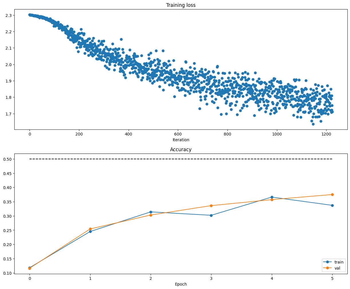
from cs231n.vis_utils import visualize_grid

# Visualize the weights of the network

def show_net_weights(net):
    W1 = net.params['W1']
    W1 = W1.reshape(3, 32, 32, -1).transpose(3, 1, 2, 0)
    plt.imshow(visualize_grid(W1, padding=3).astype('uint8'))
    plt.gca().axis('off')
    plt.show()

show_net_weights(model)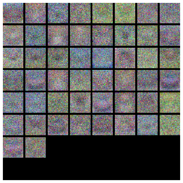
Tune your hyperparameters
What’s wrong?. Looking at the visualizations above, we see that the loss is decreasing more or less linearly, which seems to suggest that the learning rate may be too low. Moreover, there is no gap between the training and validation accuracy, suggesting that the model we used has low capacity, and that we should increase its size. On the other hand, with a very large model we would expect to see more overfitting, which would manifest itself as a very large gap between the training and validation accuracy.
Tuning. Tuning the hyperparameters and developing intuition for how they affect the final performance is a large part of using Neural Networks, so we want you to get a lot of practice. Below, you should experiment with different values of the various hyperparameters, including hidden layer size, learning rate, numer of training epochs, and regularization strength. You might also consider tuning the learning rate decay, but you should be able to get good performance using the default value.
Approximate results. You should be aim to achieve a classification accuracy of greater than 48% on the validation set. Our best network gets over 52% on the validation set.
Experiment: You goal in this exercise is to get as good of a result on CIFAR-10 as you can (52% could serve as a reference), with a fully-connected Neural Network. Feel free implement your own techniques (e.g. PCA to reduce dimensionality, or adding dropout, or adding features to the solver, etc.).
best_model = None

import itertools
import warnings
warnings.filterwarnings("ignore")

#################################################################################
# TODO: Tune hyperparameters using the validation set. Store your best trained  #
# model in best_model.                                                          #
#                                                                               #
# To help debug your network, it may help to use visualizations similar to the  #
# ones we used above; these visualizations will have significant qualitative    #
# differences from the ones we saw above for the poorly tuned network.          #
#                                                                               #
# Tweaking hyperparameters by hand can be fun, but you might find it useful to  #
# write code to sweep through possible combinations of hyperparameters          #
# automatically like we did on thexs previous exercises.                          #
#################################################################################
# *****START OF YOUR CODE (DO NOT DELETE/MODIFY THIS LINE)*****
best_solver = None
best_combination = None

input_size = 32 * 32 * 3
num_classes = 10

results = {}
best_val = -1   # The highest validation accuracy that we have seen so far.

hidden_sizes = [100, 250, 500]
num_epochs_list = [5, 9, 15]
learning_rates = [1e-2, 5e-2 ,1e-3]
reg_strength = [0.5, 0.7, 0.9]


# *****START OF YOUR CODE (DO NOT DELETE/MODIFY THIS LINE)*****

searching_list = list(itertools.product(hidden_sizes, num_epochs_list,
                                        learning_rates, reg_strength))

grid_search_start = time.time()
for combination in searching_list:

  hidden_size, num_epochs, learning_rate, reg_strength= combination
  print('hidden_size:{}, num_epochs:{}, learning_rate:{}, reg_strength:{}'.
        format(hidden_size, num_epochs, learning_rate, reg_strength))

  model = TwoLayerNet(input_size, hidden_size, num_classes, reg=reg_strength)
  solver = Solver(model, data, update_rule='sgd', lr_decay = 0.95,
                  optim_config={
                      'learning_rate': learning_rate
                  },
                  num_epochs=num_epochs, batch_size=200, print_every=-1, verbose=False
  )
  tic = time.time()
  solver.train()
  toc = time.time()
  elapsed_time = toc-tic
  print('\ttraining_time:{}, val_acc:{}'.format(round(elapsed_time, 2), solver.val_acc_history[-1]))

  results[combination] = [solver.loss_history, solver.train_acc_history,
                          solver.val_acc_history]

  if solver.val_acc_history[-1] > best_val:
    best_val = solver.val_acc_history[-1]
    best_solver = solver
    best_model = model
    best_combination = combination

  print('-----------------------------------\n')

grid_search_end = time.time()
elapsed_time = grid_search_end- grid_search_start
print('Total Grid Search Time:{}'.format(round(elapsed_time, 2)))

# *****END OF YOUR CODE (DO NOT DELETE/MODIFY THIS LINE)*****
################################################################################
#                              END OF YOUR CODE                                #
################################################################################
hidden_size:100, num_epochs:5, learning_rate:0.01, reg_strength:0.5
training_time:23.98
-----------------------------------
hidden_size:100, num_epochs:5, learning_rate:0.01, reg_strength:0.7
training_time:18.69
-----------------------------------
hidden_size:100, num_epochs:5, learning_rate:0.01, reg_strength:0.9
training_time:20.32
-----------------------------------
hidden_size:100, num_epochs:5, learning_rate:0.05, reg_strength:0.5
training_time:19.33
-----------------------------------
hidden_size:100, num_epochs:5, learning_rate:0.05, reg_strength:0.7
training_time:19.93
-----------------------------------
hidden_size:100, num_epochs:5, learning_rate:0.05, reg_strength:0.9
training_time:18.7
-----------------------------------
hidden_size:100, num_epochs:5, learning_rate:0.001, reg_strength:0.5
training_time:20.22
-----------------------------------
hidden_size:100, num_epochs:5, learning_rate:0.001, reg_strength:0.7
training_time:19.0
-----------------------------------
hidden_size:100, num_epochs:5, learning_rate:0.001, reg_strength:0.9
training_time:20.28
-----------------------------------
hidden_size:100, num_epochs:9, learning_rate:0.01, reg_strength:0.5
training_time:34.45
-----------------------------------
hidden_size:100, num_epochs:9, learning_rate:0.01, reg_strength:0.7
training_time:36.69
-----------------------------------
hidden_size:100, num_epochs:9, learning_rate:0.01, reg_strength:0.9
training_time:37.46
-----------------------------------
hidden_size:100, num_epochs:9, learning_rate:0.05, reg_strength:0.5
training_time:34.82
-----------------------------------
hidden_size:100, num_epochs:9, learning_rate:0.05, reg_strength:0.7
training_time:35.66
-----------------------------------
hidden_size:100, num_epochs:9, learning_rate:0.05, reg_strength:0.9
training_time:35.63
-----------------------------------
hidden_size:100, num_epochs:9, learning_rate:0.001, reg_strength:0.5
training_time:36.15
-----------------------------------
hidden_size:100, num_epochs:9, learning_rate:0.001, reg_strength:0.7
training_time:35.21
-----------------------------------
hidden_size:100, num_epochs:9, learning_rate:0.001, reg_strength:0.9
training_time:35.69
-----------------------------------
hidden_size:100, num_epochs:15, learning_rate:0.01, reg_strength:0.5
training_time:57.41
-----------------------------------
hidden_size:100, num_epochs:15, learning_rate:0.01, reg_strength:0.7
training_time:58.69
-----------------------------------
hidden_size:100, num_epochs:15, learning_rate:0.01, reg_strength:0.9
training_time:58.59
-----------------------------------
hidden_size:100, num_epochs:15, learning_rate:0.05, reg_strength:0.5
training_time:58.16
-----------------------------------
hidden_size:100, num_epochs:15, learning_rate:0.05, reg_strength:0.7
training_time:59.25
-----------------------------------
hidden_size:100, num_epochs:15, learning_rate:0.05, reg_strength:0.9
training_time:57.97
-----------------------------------
hidden_size:100, num_epochs:15, learning_rate:0.001, reg_strength:0.5
training_time:59.55
-----------------------------------
hidden_size:100, num_epochs:15, learning_rate:0.001, reg_strength:0.7
training_time:57.41
-----------------------------------
hidden_size:100, num_epochs:15, learning_rate:0.001, reg_strength:0.9
training_time:58.81
-----------------------------------
hidden_size:250, num_epochs:5, learning_rate:0.01, reg_strength:0.5
training_time:42.94
-----------------------------------
hidden_size:250, num_epochs:5, learning_rate:0.01, reg_strength:0.7
training_time:41.87
-----------------------------------
hidden_size:250, num_epochs:5, learning_rate:0.01, reg_strength:0.9
training_time:41.82
-----------------------------------
hidden_size:250, num_epochs:5, learning_rate:0.05, reg_strength:0.5
training_time:41.52
-----------------------------------
hidden_size:250, num_epochs:5, learning_rate:0.05, reg_strength:0.7
training_time:42.16
-----------------------------------
hidden_size:250, num_epochs:5, learning_rate:0.05, reg_strength:0.9
training_time:42.45
-----------------------------------
hidden_size:250, num_epochs:5, learning_rate:0.001, reg_strength:0.5
training_time:42.06
-----------------------------------
hidden_size:250, num_epochs:5, learning_rate:0.001, reg_strength:0.7
training_time:43.54
-----------------------------------
hidden_size:250, num_epochs:5, learning_rate:0.001, reg_strength:0.9
training_time:42.59
-----------------------------------
hidden_size:250, num_epochs:9, learning_rate:0.01, reg_strength:0.5
training_time:75.63
-----------------------------------
hidden_size:250, num_epochs:9, learning_rate:0.01, reg_strength:0.7
training_time:76.77
-----------------------------------
hidden_size:250, num_epochs:9, learning_rate:0.01, reg_strength:0.9
training_time:74.67
-----------------------------------
hidden_size:250, num_epochs:9, learning_rate:0.05, reg_strength:0.5
training_time:75.83
-----------------------------------
hidden_size:250, num_epochs:9, learning_rate:0.05, reg_strength:0.7
training_time:75.45
-----------------------------------
hidden_size:250, num_epochs:9, learning_rate:0.05, reg_strength:0.9
training_time:74.01
-----------------------------------
hidden_size:250, num_epochs:9, learning_rate:0.001, reg_strength:0.5
training_time:77.19
-----------------------------------
hidden_size:250, num_epochs:9, learning_rate:0.001, reg_strength:0.7
training_time:76.26
-----------------------------------
hidden_size:250, num_epochs:9, learning_rate:0.001, reg_strength:0.9
training_time:74.68
-----------------------------------
hidden_size:250, num_epochs:15, learning_rate:0.01, reg_strength:0.5
training_time:126.17
-----------------------------------
hidden_size:250, num_epochs:15, learning_rate:0.01, reg_strength:0.7
training_time:123.78
-----------------------------------
hidden_size:250, num_epochs:15, learning_rate:0.01, reg_strength:0.9
training_time:126.33
-----------------------------------
hidden_size:250, num_epochs:15, learning_rate:0.05, reg_strength:0.5
training_time:124.37
-----------------------------------
hidden_size:250, num_epochs:15, learning_rate:0.05, reg_strength:0.7
training_time:125.64
-----------------------------------
hidden_size:250, num_epochs:15, learning_rate:0.05, reg_strength:0.9
training_time:125.73
-----------------------------------
hidden_size:250, num_epochs:15, learning_rate:0.001, reg_strength:0.5
training_time:126.37
-----------------------------------
hidden_size:250, num_epochs:15, learning_rate:0.001, reg_strength:0.7
training_time:126.6
-----------------------------------
hidden_size:250, num_epochs:15, learning_rate:0.001, reg_strength:0.9
training_time:125.85
-----------------------------------
hidden_size:500, num_epochs:5, learning_rate:0.01, reg_strength:0.5
training_time:79.22
-----------------------------------
hidden_size:500, num_epochs:5, learning_rate:0.01, reg_strength:0.7
training_time:80.11
-----------------------------------
hidden_size:500, num_epochs:5, learning_rate:0.01, reg_strength:0.9
training_time:78.91
-----------------------------------
hidden_size:500, num_epochs:5, learning_rate:0.05, reg_strength:0.5
training_time:78.52
-----------------------------------
hidden_size:500, num_epochs:5, learning_rate:0.05, reg_strength:0.7
training_time:79.89
-----------------------------------
hidden_size:500, num_epochs:5, learning_rate:0.05, reg_strength:0.9
training_time:78.77
-----------------------------------
hidden_size:500, num_epochs:5, learning_rate:0.001, reg_strength:0.5
training_time:80.77
-----------------------------------
hidden_size:500, num_epochs:5, learning_rate:0.001, reg_strength:0.7
training_time:79.28
-----------------------------------
hidden_size:500, num_epochs:5, learning_rate:0.001, reg_strength:0.9
training_time:79.07
-----------------------------------
hidden_size:500, num_epochs:9, learning_rate:0.01, reg_strength:0.5
training_time:144.07
-----------------------------------
hidden_size:500, num_epochs:9, learning_rate:0.01, reg_strength:0.7
training_time:145.36
-----------------------------------
hidden_size:500, num_epochs:9, learning_rate:0.01, reg_strength:0.9
training_time:142.78
-----------------------------------
hidden_size:500, num_epochs:9, learning_rate:0.05, reg_strength:0.5
training_time:144.7
-----------------------------------
hidden_size:500, num_epochs:9, learning_rate:0.05, reg_strength:0.7
training_time:143.2
-----------------------------------
hidden_size:500, num_epochs:9, learning_rate:0.05, reg_strength:0.9
training_time:143.46
-----------------------------------
hidden_size:500, num_epochs:9, learning_rate:0.001, reg_strength:0.5
training_time:146.41
-----------------------------------
hidden_size:500, num_epochs:9, learning_rate:0.001, reg_strength:0.7
training_time:145.12
-----------------------------------
hidden_size:500, num_epochs:9, learning_rate:0.001, reg_strength:0.9
training_time:145.96
-----------------------------------
hidden_size:500, num_epochs:15, learning_rate:0.01, reg_strength:0.5
training_time:238.95
-----------------------------------
hidden_size:500, num_epochs:15, learning_rate:0.01, reg_strength:0.7
training_time:239.56
-----------------------------------
hidden_size:500, num_epochs:15, learning_rate:0.01, reg_strength:0.9
training_time:239.07
-----------------------------------
hidden_size:500, num_epochs:15, learning_rate:0.05, reg_strength:0.5
training_time:239.73
-----------------------------------
hidden_size:500, num_epochs:15, learning_rate:0.05, reg_strength:0.7
training_time:239.83
-----------------------------------
hidden_size:500, num_epochs:15, learning_rate:0.05, reg_strength:0.9
training_time:239.73
-----------------------------------
hidden_size:500, num_epochs:15, learning_rate:0.001, reg_strength:0.5
training_time:240.77
-----------------------------------
hidden_size:500, num_epochs:15, learning_rate:0.001, reg_strength:0.7
training_time:240.77
-----------------------------------
hidden_size:500, num_epochs:15, learning_rate:0.001, reg_strength:0.9
training_time:240.49
-----------------------------------
Total Grid Search Time:7397.71print('best_combination:')
hidden_size, num_epochs, learning_rate, reg_strength= combination
print('\thidden_size:{}, num_epochs:{}, learning_rate:{}, reg_strength:{}'.
format(hidden_size, num_epochs, learning_rate, reg_strength))Test your model!
Run your best model on the validation and test sets. You should achieve above 48% accuracy on the validation set and the test set.
y_val_pred = np.argmax(best_model.loss(data['X_val']), axis=1)
print('Validation set accuracy: ', (y_val_pred == data['y_val']).mean())
Validation set accuracy: 0.552y_test_pred = np.argmax(best_model.loss(data['X_test']), axis=1)
print('Test set accuracy: ', (y_test_pred == data['y_test']).mean())Test set accuracy: 0.547Inline Question 2:
Now that you have trained a Neural Network classifier, you may find that your testing accuracy is much lower than the training accuracy. In what ways can we decrease this gap? Select all that apply.
- Train on a larger dataset.
- Add more hidden units.
- Increase the regularization strength.
- None of the above.
\(\color{blue}{\textit Your Answer:}\)
\(\color{blue}{\textit Your Explanation:}\)