CS231N

This course is a deep dive into the details of deep learning architectures with a focus on learning end-to-end models for these tasks, particularly image classification

This page contains my solutions and approaches for the assignment All source codes of my solutions are available on GitHub

Image features exercise

Complete and hand in this completed worksheet (including its outputs and any supporting code outside of the worksheet) with your assignment submission. For more details see the assignments page on the course website.

We have seen that we can achieve reasonable performance on an image classification task by training a linear classifier on the pixels of the input image. In this exercise we will show that we can improve our classification performance by training linear classifiers not on raw pixels but on features that are computed from the raw pixels.

All of your work for this exercise will be done in this notebook.

import random
import numpy as np
from cs231n.data_utils import load_CIFAR10
import matplotlib.pyplot as plt


%matplotlib inline
plt.rcParams['figure.figsize'] = (10.0, 8.0) # set default size of plots
plt.rcParams['image.interpolation'] = 'nearest'
plt.rcParams['image.cmap'] = 'gray'

# for auto-reloading extenrnal modules
# see http://stackoverflow.com/questions/1907993/autoreload-of-modules-in-ipython
%load_ext autoreload
%autoreload 2

Load data

Similar to previous exercises, we will load CIFAR-10 data from disk.

from cs231n.features import color_histogram_hsv, hog_feature

def get_CIFAR10_data(num_training=49000, num_validation=1000, num_test=1000):
    # Load the raw CIFAR-10 data
    cifar10_dir = 'cs231n/datasets/cifar-10-batches-py'

    # Cleaning up variables to prevent loading data multiple times (which may cause memory issue)
    try:
       del X_train, y_train
       del X_test, y_test
       print('Clear previously loaded data.')
    except:
       pass

    X_train, y_train, X_test, y_test = load_CIFAR10(cifar10_dir)
    
    # Subsample the data
    mask = list(range(num_training, num_training + num_validation))
    X_val = X_train[mask]
    y_val = y_train[mask]
    mask = list(range(num_training))
    X_train = X_train[mask]
    y_train = y_train[mask]
    mask = list(range(num_test))
    X_test = X_test[mask]
    y_test = y_test[mask]
    
    return X_train, y_train, X_val, y_val, X_test, y_test

X_train, y_train, X_val, y_val, X_test, y_test = get_CIFAR10_data()

Extract Features

For each image we will compute a Histogram of Oriented Gradients (HOG) as well as a color histogram using the hue channel in HSV color space. We form our final feature vector for each image by concatenating the HOG and color histogram feature vectors.

Roughly speaking, HOG should capture the texture of the image while ignoring color information, and the color histogram represents the color of the input image while ignoring texture. As a result, we expect that using both together ought to work better than using either alone. Verifying this assumption would be a good thing to try for your own interest.

The hog_feature and color_histogram_hsv functions both operate on a single image and return a feature vector for that image. The extract_features function takes a set of images and a list of feature functions and evaluates each feature function on each image, storing the results in a matrix where each column is the concatenation of all feature vectors for a single image.

from cs231n.features import *

num_color_bins = 10 # Number of bins in the color histogram
feature_fns = [hog_feature, lambda img: color_histogram_hsv(img, nbin=num_color_bins)]
X_train_feats = extract_features(X_train, feature_fns, verbose=True)
X_val_feats = extract_features(X_val, feature_fns)
X_test_feats = extract_features(X_test, feature_fns)

# Preprocessing: Subtract the mean feature
mean_feat = np.mean(X_train_feats, axis=0, keepdims=True)
X_train_feats -= mean_feat
X_val_feats -= mean_feat
X_test_feats -= mean_feat

# Preprocessing: Divide by standard deviation. This ensures that each feature
# has roughly the same scale.
std_feat = np.std(X_train_feats, axis=0, keepdims=True)
X_train_feats /= std_feat
X_val_feats /= std_feat
X_test_feats /= std_feat

# Preprocessing: Add a bias dimension
X_train_feats = np.hstack([X_train_feats, np.ones((X_train_feats.shape[0], 1))])
X_val_feats = np.hstack([X_val_feats, np.ones((X_val_feats.shape[0], 1))])
X_test_feats = np.hstack([X_test_feats, np.ones((X_test_feats.shape[0], 1))])

Done extracting features for 1000 / 49000 images
Done extracting features for 2000 / 49000 images
Done extracting features for 3000 / 49000 images
Done extracting features for 4000 / 49000 images
Done extracting features for 5000 / 49000 images
Done extracting features for 6000 / 49000 images
Done extracting features for 7000 / 49000 images
Done extracting features for 8000 / 49000 images
Done extracting features for 9000 / 49000 images
Done extracting features for 10000 / 49000 images
Done extracting features for 11000 / 49000 images
Done extracting features for 12000 / 49000 images
Done extracting features for 13000 / 49000 images
Done extracting features for 14000 / 49000 images
Done extracting features for 15000 / 49000 images
Done extracting features for 16000 / 49000 images
Done extracting features for 17000 / 49000 images
Done extracting features for 18000 / 49000 images
Done extracting features for 19000 / 49000 images
Done extracting features for 20000 / 49000 images
Done extracting features for 21000 / 49000 images
Done extracting features for 22000 / 49000 images
Done extracting features for 23000 / 49000 images
Done extracting features for 24000 / 49000 images
Done extracting features for 25000 / 49000 images
Done extracting features for 26000 / 49000 images
Done extracting features for 27000 / 49000 images
Done extracting features for 28000 / 49000 images
Done extracting features for 29000 / 49000 images
Done extracting features for 30000 / 49000 images
Done extracting features for 31000 / 49000 images
Done extracting features for 32000 / 49000 images
Done extracting features for 33000 / 49000 images
Done extracting features for 34000 / 49000 images
Done extracting features for 35000 / 49000 images
Done extracting features for 36000 / 49000 images
Done extracting features for 37000 / 49000 images
Done extracting features for 38000 / 49000 images
Done extracting features for 39000 / 49000 images
Done extracting features for 40000 / 49000 images
Done extracting features for 41000 / 49000 images
Done extracting features for 42000 / 49000 images
Done extracting features for 43000 / 49000 images
Done extracting features for 44000 / 49000 images
Done extracting features for 45000 / 49000 images
Done extracting features for 46000 / 49000 images
Done extracting features for 47000 / 49000 images
Done extracting features for 48000 / 49000 images
Done extracting features for 49000 / 49000 images

Train SVM on features

Using the multiclass SVM code developed earlier in the assignment, train SVMs on top of the features extracted above; this should achieve better results than training SVMs directly on top of raw pixels.

# Use the validation set to tune the learning rate and regularization strength

from cs231n.classifiers.linear_classifier import LinearSVM

learning_rates = [1e-9, 1e-8, 1e-7]
regularization_strengths = [5e4, 5e5, 5e6]

results = {}
best_val = -1
best_svm = None

################################################################################
# TODO:                                                                        #
# Use the validation set to set the learning rate and regularization strength. #
# This should be identical to the validation that you did for the SVM; save    #
# the best trained classifer in best_svm. You might also want to play          #
# with different numbers of bins in the color histogram. If you are careful    #
# you should be able to get accuracy of near 0.44 on the validation set.       #
################################################################################
# *****START OF YOUR CODE (DO NOT DELETE/MODIFY THIS LINE)*****

import itertools
for lr, reg in itertools.product(learning_rates, regularization_strengths):
  svm = LinearSVM()
  loss_hist = svm.train(X_train_feats, y_train, learning_rate=lr, reg=reg,
                        num_iters=1500, verbose=False)
  y_train_pred = svm.predict(X_train_feats)
  train_accuracy = np.mean(y_train == y_train_pred)
  y_val_pred = svm.predict(X_val_feats)
  val_accuracy  = np.mean(y_val == y_val_pred)

  results[(lr, reg)] = train_accuracy, val_accuracy
  if val_accuracy > best_val:
    best_val = val_accuracy
    best_svm = svm

# *****END OF YOUR CODE (DO NOT DELETE/MODIFY THIS LINE)*****

# Print out results.
for lr, reg in sorted(results):
    train_accuracy, val_accuracy = results[(lr, reg)]
    print('lr %e reg %e train accuracy: %f val accuracy: %f' % (
                lr, reg, train_accuracy, val_accuracy))
    
print('best validation accuracy achieved: %f' % best_val)

lr 1.000000e-09 reg 5.000000e+04 train accuracy: 0.107510 val accuracy: 0.111000
lr 1.000000e-09 reg 5.000000e+05 train accuracy: 0.096857 val accuracy: 0.101000
lr 1.000000e-09 reg 5.000000e+06 train accuracy: 0.414286 val accuracy: 0.418000
lr 1.000000e-08 reg 5.000000e+04 train accuracy: 0.112306 val accuracy: 0.153000
lr 1.000000e-08 reg 5.000000e+05 train accuracy: 0.415184 val accuracy: 0.407000
lr 1.000000e-08 reg 5.000000e+06 train accuracy: 0.416592 val accuracy: 0.417000
lr 1.000000e-07 reg 5.000000e+04 train accuracy: 0.414816 val accuracy: 0.423000
lr 1.000000e-07 reg 5.000000e+05 train accuracy: 0.409122 val accuracy: 0.412000
lr 1.000000e-07 reg 5.000000e+06 train accuracy: 0.326061 val accuracy: 0.339000
best validation accuracy achieved: 0.423000

# Evaluate your trained SVM on the test set: you should be able to get at least 0.40
y_test_pred = best_svm.predict(X_test_feats)
test_accuracy = np.mean(y_test == y_test_pred)
print(test_accuracy)

0.417

# An important way to gain intuition about how an algorithm works is to
# visualize the mistakes that it makes. In this visualization, we show examples
# of images that are misclassified by our current system. The first column
# shows images that our system labeled as "plane" but whose true label is
# something other than "plane".

examples_per_class = 8
classes = ['plane', 'car', 'bird', 'cat', 'deer', 'dog', 'frog', 'horse', 'ship', 'truck']
for cls, cls_name in enumerate(classes):
    idxs = np.where((y_test != cls) & (y_test_pred == cls))[0]
    idxs = np.random.choice(idxs, examples_per_class, replace=False)
    for i, idx in enumerate(idxs):
        plt.subplot(examples_per_class, len(classes), i * len(classes) + cls + 1)
        plt.imshow(X_test[idx].astype('uint8'))
        plt.axis('off')
        if i == 0:
            plt.title(cls_name)
plt.show()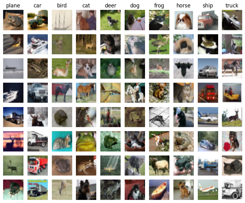

Inline question 1:

Describe the misclassification results that you see. Do they make sense?

\(\color{blue}{\textit Your Answer:}\)

Neural Network on image features

Earlier in this assigment we saw that training a two-layer neural network on raw pixels achieved better classification performance than linear classifiers on raw pixels. In this notebook we have seen that linear classifiers on image features outperform linear classifiers on raw pixels.

For completeness, we should also try training a neural network on image features. This approach should outperform all previous approaches: you should easily be able to achieve over 55% classification accuracy on the test set; our best model achieves about 60% classification accuracy.

# Preprocessing: Remove the bias dimension
# Make sure to run this cell only ONCE
print(X_train_feats.shape)
X_train_feats = X_train_feats[:, :-1]
X_val_feats = X_val_feats[:, :-1]
X_test_feats = X_test_feats[:, :-1]

print(X_train_feats.shape)

(49000, 155)
(49000, 154)

from cs231n.classifiers.fc_net import TwoLayerNet
from cs231n.solver import Solver
import time
import itertools
import warnings
import copy
warnings.filterwarnings("ignore")

input_dim = X_train_feats.shape[1]
hidden_dim = 500
num_classes = 10

data = {
    'X_train': X_train_feats, 
    'y_train': y_train, 
    'X_val': X_val_feats, 
    'y_val': y_val, 
    'X_test': X_test_feats, 
    'y_test': y_test, 
}

net = TwoLayerNet(input_dim, hidden_dim, num_classes)
best_model = None

################################################################################
# TODO: Train a two-layer neural network on image features. You may want to    #
# cross-validate various parameters as in previous sections. Store your best   #
# model in the best_net variable.                                              #
################################################################################
# *****START OF YOUR CODE (DO NOT DELETE/MODIFY THIS LINE)*****

results = {}
best_val = -1

learning_rates = np.linspace(1e-2, 2.75e-2, 4)
regularization_strengths = np.geomspace(1e-6, 1e-4, 3)

data = {
    'X_train': X_train_feats,
    'X_val': X_val_feats,
    'X_test': X_test_feats,
    'y_train': y_train,
    'y_val': y_val,
    'y_test': y_test
}

import itertools

for lr, reg in itertools.product(learning_rates, regularization_strengths):
    # Create Two Layer Net and train it with Solver
    model = TwoLayerNet(input_dim, hidden_dim, num_classes)
    solver = Solver(model, data, optim_config={'learning_rate': lr}, num_epochs=15, verbose=False)
    solver.train()
    
    # Compute validation set accuracy and append to the dictionary
    results[(lr, reg)] = solver.best_val_acc

    # Save if validation accuracy is the best
    if results[(lr, reg)] > best_val:
        best_val = results[(lr, reg)]
        best_net = model

# Print out results.
for lr, reg in sorted(results):
    val_accuracy = results[(lr, reg)]
    print('lr %e reg %e val accuracy: %f' % (lr, reg, val_accuracy))
    
print('best validation accuracy achieved during cross-validation: %f' % best_val)


# *****END OF YOUR CODE (DO NOT DELETE/MODIFY THIS LINE)*****

lr 1.000000e-02 reg 1.000000e-06 val accuracy: 0.518000
lr 1.000000e-02 reg 1.000000e-05 val accuracy: 0.517000
lr 1.000000e-02 reg 1.000000e-04 val accuracy: 0.517000
lr 1.583333e-02 reg 1.000000e-06 val accuracy: 0.530000
lr 1.583333e-02 reg 1.000000e-05 val accuracy: 0.527000
lr 1.583333e-02 reg 1.000000e-04 val accuracy: 0.534000
lr 2.166667e-02 reg 1.000000e-06 val accuracy: 0.554000
lr 2.166667e-02 reg 1.000000e-05 val accuracy: 0.549000
lr 2.166667e-02 reg 1.000000e-04 val accuracy: 0.552000
lr 2.750000e-02 reg 1.000000e-06 val accuracy: 0.571000
lr 2.750000e-02 reg 1.000000e-05 val accuracy: 0.572000
lr 2.750000e-02 reg 1.000000e-04 val accuracy: 0.562000
best validation accuracy achieved during cross-validation: 0.572000

# Run your best neural net classifier on the test set. You should be able
# to get more than 55% accuracy.

y_test_pred = np.argmax(best_net.loss(data['X_test']), axis=1)
test_acc = (y_test_pred == data['y_test']).mean()
print(test_acc)

0.548