This course is a deep dive into the details of deep learning architectures with a focus on learning end-to-end models for these tasks, particularly image classification
This page contains my solutions and approaches for the assignment All source codes of my solutions are available on GitHub
Multi-Layer Fully Connected Network
In this exercise, you will implement a fully connected network with an arbitrary number of hidden layers.
Read through the FullyConnectedNet class in the file cs231n/classifiers/fc_net.py.
Implement the network initialization, forward pass, and backward pass. Throughout this assignment, you will be implementing layers in cs231n/layers.py. You can re-use your implementations for affine_forward, affine_backward, relu_forward, relu_backward, and softmax_loss from Assignment 1. For right now, don’t worry about implementing dropout or batch/layer normalization yet, as you will add those features later.
from builtins importrangefrom builtins importobjectimport numpy as npfrom ..layers import*from ..layer_utils import*class FullyConnectedNet(object):"""Class for a multi-layer fully connected neural network. Network contains an arbitrary number of hidden layers, ReLU nonlinearities, and a softmax loss function. This will also implement dropout and batch/layer normalization as options. For a network with L layers, the architecture will be {affine - [batch/layer norm] - relu - [dropout]} x (L - 1) - affine - softmax where batch/layer normalization and dropout are optional and the {...} block is repeated L - 1 times. Learnable parameters are stored in the self.params dictionary and will be learned using the Solver class. """def__init__(self, hidden_dims, input_dim=3*32*32, num_classes=10, dropout_keep_ratio=1, normalization=None, reg=0.0, weight_scale=1e-2, dtype=np.float32, seed=None, ):"""Initialize a new FullyConnectedNet. Inputs: - hidden_dims: A list of integers giving the size of each hidden layer. - input_dim: An integer giving the size of the input. - num_classes: An integer giving the number of classes to classify. - dropout_keep_ratio: Scalar between 0 and 1 giving dropout strength. If dropout_keep_ratio=1 then the network should not use dropout at all. - normalization: What type of normalization the network should use. Valid values are "batchnorm", "layernorm", or None for no normalization (the default). - reg: Scalar giving L2 regularization strength. - weight_scale: Scalar giving the standard deviation for random initialization of the weights. - dtype: A numpy datatype object; all computations will be performed using this datatype. float32 is faster but less accurate, so you should use float64 for numeric gradient checking. - seed: If not None, then pass this random seed to the dropout layers. This will make the dropout layers deteriminstic so we can gradient check the model. """self.normalization = normalizationself.use_dropout = dropout_keep_ratio !=1self.reg = regself.num_layers =1+len(hidden_dims)self.dtype = dtypeself.params = {}############################################################################# TODO: Initialize the parameters of the network, storing all values in ## the self.params dictionary. Store weights and biases for the first layer ## in W1 and b1; for the second layer use W2 and b2, etc. Weights should be ## initialized from a normal distribution centered at 0 with standard ## deviation equal to weight_scale. Biases should be initialized to zero. ## ## When using batch normalization, store scale and shift parameters for the ## first layer in gamma1 and beta1; for the second layer use gamma2 and ## beta2, etc. Scale parameters should be initialized to ones and shift ## parameters should be initialized to zeros. ############################################################################## *****START OF YOUR CODE (DO NOT DELETE/MODIFY THIS LINE)***** verbose =Falseif verbose: print('num_layers:', self.num_layers, '\n') len_hidden_dims =len(hidden_dims)for layer_num inrange(1, self.num_layers+1): number_of_nodes =Noneif verbose: print('layer_num:', layer_num)if layer_num ==1: # First Layerif verbose: print('\tfirst_layer')self.params[f"W{layer_num}"] = np.random.normal(0.0, weight_scale, (input_dim, hidden_dims[0]))self.params[f"b{layer_num}"] = np.zeros(hidden_dims[0], )ifself.normalization =="batchnorm":self.params[f"gamma{layer_num}"] = np.ones((hidden_dims[0], ))self.params[f"beta{layer_num}"] = np.zeros((hidden_dims[0], ))elif layer_num ==self.num_layers: #Last Layerif verbose: print('\tlast_layer')self.params[f"W{layer_num}"] = np.random.normal(0.0, weight_scale, (hidden_dims[-1], num_classes))self.params[f"b{layer_num}"] = np.zeros(num_classes, )else: # Hidden Layersif verbose: print('\thidden_layer') hidden_dim_curr = hidden_dims[layer_num-2] hidden_dim_next = hidden_dims[layer_num-1]self.params[f"W{layer_num}"] = np.random.normal(0.0, weight_scale, (hidden_dim_curr, hidden_dim_next))self.params[f"b{layer_num}"] = np.zeros(hidden_dim_next, )ifself.normalization =="batchnorm":self.params[f"gamma{layer_num}"] = np.ones((hidden_dim_next, ))self.params[f"beta{layer_num}"] = np.zeros((hidden_dim_next, ))if verbose: print(f"\tW{layer_num}:", self.params[f"W{layer_num}"].shape)print(f"\tb{layer_num}:", self.params[f"b{layer_num}"].shape)iff"gamma{layer_num}"inself.params:print(f"\tgamma{layer_num}:", self.params[f"gamma{layer_num}"].shape)print(f"\tbeta{layer_num}:", self.params[f"beta{layer_num}"].shape)# *****END OF YOUR CODE (DO NOT DELETE/MODIFY THIS LINE)*****############################################################################# END OF YOUR CODE ############################################################################## When using dropout we need to pass a dropout_param dictionary to each# dropout layer so that the layer knows the dropout probability and the mode# (train / test). You can pass the same dropout_param to each dropout layer.self.dropout_param = {}ifself.use_dropout:self.dropout_param = {"mode": "train", "p": dropout_keep_ratio}if seed isnotNone:self.dropout_param["seed"] = seed# With batch normalization we need to keep track of running means and# variances, so we need to pass a special bn_param object to each batch# normalization layer. You should pass self.bn_params[0] to the forward pass# of the first batch normalization layer, self.bn_params[1] to the forward# pass of the second batch normalization layer, etc.self.bn_params = []ifself.normalization =="batchnorm":self.bn_params = [{"mode": "train"} for i inrange(self.num_layers -1)]ifself.normalization =="layernorm":self.bn_params = [{} for i inrange(self.num_layers -1)]# Cast all parameters to the correct datatype.for k, v inself.params.items():self.params[k] = v.astype(dtype)def loss(self, X, y=None):"""Compute loss and gradient for the fully connected net. Inputs: - X: Array of input data of shape (N, d_1, ..., d_k) - y: Array of labels, of shape (N,). y[i] gives the label for X[i]. Returns: If y is None, then run a test-time forward pass of the model and return: - scores: Array of shape (N, C) giving classification scores, where scores[i, c] is the classification score for X[i] and class c. If y is not None, then run a training-time forward and backward pass and return a tuple of: - loss: Scalar value giving the loss - grads: Dictionary with the same keys as self.params, mapping parameter names to gradients of the loss with respect to those parameters. """ X = X.astype(self.dtype) mode ="test"if y isNoneelse"train"# Set train/test mode for batchnorm params and dropout param since they# behave differently during training and testing.ifself.use_dropout:self.dropout_param["mode"] = modeifself.normalization =="batchnorm":for bn_param inself.bn_params: bn_param["mode"] = mode scores =None############################################################################# TODO: Implement the forward pass for the fully connected net, computing ## the class scores for X and storing them in the scores variable. ## ## When using dropout, you'll need to pass self.dropout_param to each ## dropout forward pass. ## ## When using batch normalization, you'll need to pass self.bn_params[0] to ## the forward pass for the first batch normalization layer, pass ## self.bn_params[1] to the forward pass for the second batch normalization ## layer, etc. ############################################################################## *****START OF YOUR CODE (DO NOT DELETE/MODIFY THIS LINE)***** affine_cache =None bn_cache =None relu_cache =None dropout_cache =None caches = {} input_data = Xfor layer_num inrange(1, self.num_layers): weights =self.params[f"W{layer_num}"] biases =self.params[f"b{layer_num}"] temp_out, affine_cache = affine_forward(input_data, weights, biases)#batch/layer normifself.normalization =="batchnorm": x = temp_out gamma =self.params[f"gamma{layer_num}"] beta =self.params[f"beta{layer_num}"] bn_param =self.bn_params[layer_num-1] temp_out, bn_cache = batchnorm_forward(x, gamma, beta, bn_param) relu_out, relu_cache = relu_forward(temp_out)#dropout input_data = relu_out cache = (affine_cache, bn_cache, relu_cache, dropout_cache) caches[f"cache{layer_num}"] = cache layer_num =self.num_layers weights =self.params[f"W{layer_num}"] biases =self.params[f"b{layer_num}"] affine_out, affine_cache = affine_forward(input_data, weights, biases) caches[f"cache{layer_num}"] = affine_cache scores = affine_out# *****END OF YOUR CODE (DO NOT DELETE/MODIFY THIS LINE)*****############################################################################# END OF YOUR CODE ############################################################################## If test mode return early.if mode =="test":return scores loss, grads =0.0, {}############################################################################# TODO: Implement the backward pass for the fully connected net. Store the ## loss in the loss variable and gradients in the grads dictionary. Compute ## data loss using softmax, and make sure that grads[k] holds the gradients ## for self.params[k]. Don't forget to add L2 regularization! ## ## When using batch/layer normalization, you don't need to regularize the ## scale and shift parameters. ## ## NOTE: To ensure that your implementation matches ours and you pass the ## automated tests, make sure that your L2 regularization includes a factor ## of 0.5 to simplify the expression for the gradient. ############################################################################## *****START OF YOUR CODE (DO NOT DELETE/MODIFY THIS LINE)***** loss, dout = softmax_loss(scores, y) layer_num =self.num_layers w =self.params[f"W{layer_num}"] cache = caches[f"cache{layer_num}"] dx, dw, db = affine_backward(dout, cache) grads[f"W{layer_num}"] = dw + (self.reg * w) grads[f"b{layer_num}"] = db loss +=0.5*self.reg * (np.sum(w * w))for layer_num inrange(self.num_layers-1, 0, -1): cache = caches[f"cache{layer_num}"] w =self.params[f"W{layer_num}"] affine_cache, bn_cache, relu_cache, dropout_cache = cache temp_dout = relu_backward(dx, relu_cache)ifself.normalization =="batchnorm": temp_dout, dgamma, dbeta = batchnorm_backward_alt(temp_dout, bn_cache) dx, dw, db = affine_backward(temp_dout, affine_cache) grads[f"W{layer_num}"] = dw + (self.reg *self.params[f"W{layer_num}"]) grads[f"b{layer_num}"] = dbifself.normalization =="batchnorm": grads[f"gamma{layer_num}"] = dgamma grads[f"beta{layer_num}"] = dbeta loss +=0.5*self.reg * (np.sum(w * w))# *****END OF YOUR CODE (DO NOT DELETE/MODIFY THIS LINE)*****############################################################################# END OF YOUR CODE #############################################################################return loss, grads
As a sanity check, run the following to check the initial loss and to gradient check the network both with and without regularization. This is a good way to see if the initial losses seem reasonable.
For gradient checking, you should expect to see errors around 1e-7 or less.
np.random.seed(231)N, D, H1, H2, C =2, 15, 20, 30, 10X = np.random.randn(N, D)y = np.random.randint(C, size=(N,))for reg in [0, 3.14]:print("Running check with reg = ", reg) model = FullyConnectedNet( [H1, H2], input_dim=D, num_classes=C, reg=reg, weight_scale=5e-2, dtype=np.float64 ) loss, grads = model.loss(X, y)print("Initial loss: ", loss)# Most of the errors should be on the order of e-7 or smaller. # NOTE: It is fine however to see an error for W2 on the order of e-5# for the check when reg = 0.0for name insorted(grads): f =lambda _: model.loss(X, y)[0] grad_num = eval_numerical_gradient(f, model.params[name], verbose=False, h=1e-5)print(f"{name} relative error: {rel_error(grad_num, grads[name])}")
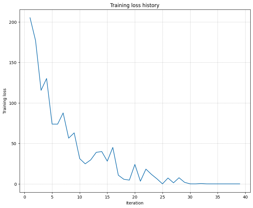
As another sanity check, make sure your network can overfit on a small dataset of 50 images. First, we will try a three-layer network with 100 units in each hidden layer. In the following cell, tweak the learning rate and weight initialization scale to overfit and achieve 100% training accuracy within 20 epochs.
# TODO: Use a three-layer Net to overfit 50 training examples by # tweaking just the learning rate and initialization scale.num_train =50small_data = {"X_train": data["X_train"][:num_train],"y_train": data["y_train"][:num_train],"X_val": data["X_val"],"y_val": data["y_val"],}weight_scale =1e-1# Experiment with this!learning_rate =1e-4# Experiment with this!model = FullyConnectedNet( [100, 100], weight_scale=weight_scale, dtype=np.float64)solver = Solver( model, small_data, print_every=10, num_epochs=20, batch_size=25, update_rule="sgd", optim_config={"learning_rate": learning_rate},)solver.train()plt.plot(solver.loss_history)plt.title("Training loss history")plt.xlabel("Iteration")plt.ylabel("Training loss")plt.grid(linestyle='--', linewidth=0.5)plt.show()
/content/drive/My Drive/Colab Notebooks/cs231n/assignments/assignment2/cs231n/layers.py:824: RuntimeWarning: divide by zero encountered in log
  loss =  - np.sum(np.log(correct_class_probs))
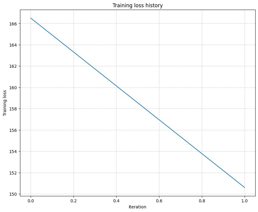
Now, try to use a five-layer network with 100 units on each layer to overfit on 50 training examples. Again, you will have to adjust the learning rate and weight initialization scale, but you should be able to achieve 100% training accuracy within 20 epochs.
# TODO: Use a five-layer Net to overfit 50 training examples by # tweaking just the learning rate and initialization scale.num_train =50small_data = {'X_train': data['X_train'][:num_train],'y_train': data['y_train'][:num_train],'X_val': data['X_val'],'y_val': data['y_val'],}learning_rate =2e-3# Experiment with this!weight_scale =1e-1# Experiment with this!model = FullyConnectedNet( [100, 100, 100, 100], weight_scale=weight_scale, dtype=np.float64)solver = Solver( model, small_data, print_every=10, num_epochs=20, batch_size=25, update_rule='sgd', optim_config={'learning_rate': learning_rate},)solver.train()plt.plot(solver.loss_history)plt.title('Training loss history')plt.xlabel('Iteration')plt.ylabel('Training loss')plt.grid(linestyle='--', linewidth=0.5)plt.show()
/content/drive/My Drive/Colab Notebooks/cs231n/assignments/assignment2/cs231n/layers.py:821: RuntimeWarning: overflow encountered in exp
  exps = np.exp(x)
/content/drive/My Drive/Colab Notebooks/cs231n/assignments/assignment2/cs231n/layers.py:822: RuntimeWarning: invalid value encountered in true_divide
  probs = exps / np.sum(exps, axis=-1, keepdims=True)
Inline Question 1:
Did you notice anything about the comparative difficulty of training the three-layer network vs. training the five-layer network? In particular, based on your experience, which network seemed more sensitive to the initialization scale? Why do you think that is the case?
Answer:
[FILL THIS IN]
Update rules
So far we have used vanilla stochastic gradient descent (SGD) as our update rule. More sophisticated update rules can make it easier to train deep networks. We will implement a few of the most commonly used update rules and compare them to vanilla SGD.
SGD+Momentum
Stochastic gradient descent with momentum is a widely used update rule that tends to make deep networks converge faster than vanilla stochastic gradient descent. See the Momentum Update section at http://cs231n.github.io/neural-networks-3/#sgd for more information.
Open the file cs231n/optim.py and read the documentation at the top of the file to make sure you understand the API. Implement the SGD+momentum update rule in the function sgd_momentum and run the following to check your implementation. You should see errors less than e-8.
def sgd_momentum(w, dw, config=None):""" Performs stochastic gradient descent with momentum. config format: - learning_rate: Scalar learning rate. - momentum: Scalar between 0 and 1 giving the momentum value. Setting momentum = 0 reduces to sgd. - velocity: A numpy array of the same shape as w and dw used to store a moving average of the gradients. """if config isNone: config = {} config.setdefault("learning_rate", 1e-2) config.setdefault("momentum", 0.9) v = config.get("velocity", np.zeros_like(w)) next_w =None############################################################################ TODO: Implement the momentum update formula. Store the updated value in ## the next_w variable. You should also use and update the velocity v. ############################################################################# *****START OF YOUR CODE (DO NOT DELETE/MODIFY THIS LINE)***** v = (config['momentum'] * v) - (config['learning_rate'] * dw) next_w = w+v # *****END OF YOUR CODE (DO NOT DELETE/MODIFY THIS LINE)*****############################################################################ END OF YOUR CODE ############################################################################ config["velocity"] = vreturn next_w, config
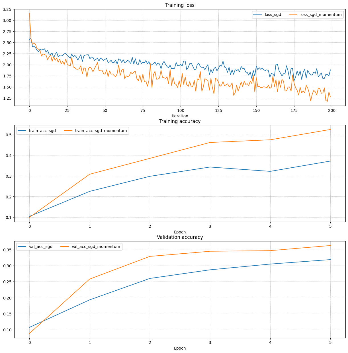
Once you have done so, run the following to train a six-layer network with both SGD and SGD+momentum. You should see the SGD+momentum update rule converge faster.
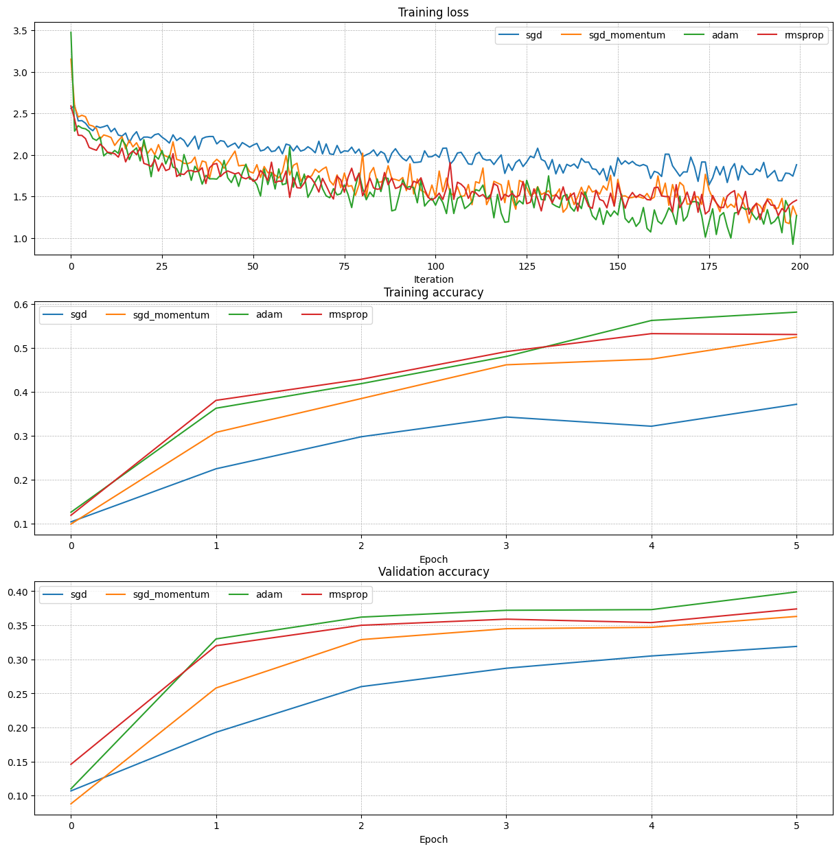
RMSProp [1] and Adam [2] are update rules that set per-parameter learning rates by using a running average of the second moments of gradients.
In the file cs231n/optim.py, implement the RMSProp update rule in the rmsprop function and implement the Adam update rule in the adam function, and check your implementations using the tests below.
NOTE: Please implement the complete Adam update rule (with the bias correction mechanism), not the first simplified version mentioned in the course notes.
[1] Tijmen Tieleman and Geoffrey Hinton. “Lecture 6.5-rmsprop: Divide the gradient by a running average of its recent magnitude.” COURSERA: Neural Networks for Machine Learning 4 (2012).
[2] Diederik Kingma and Jimmy Ba, “Adam: A Method for Stochastic Optimization”, ICLR 2015.
def rmsprop(w, dw, config=None):""" Uses the RMSProp update rule, which uses a moving average of squared gradient values to set adaptive per-parameter learning rates. config format: - learning_rate: Scalar learning rate. - decay_rate: Scalar between 0 and 1 giving the decay rate for the squared gradient cache. - epsilon: Small scalar used for smoothing to avoid dividing by zero. - cache: Moving average of second moments of gradients. """if config isNone: config = {} config.setdefault("learning_rate", 1e-2) config.setdefault("decay_rate", 0.99) config.setdefault("epsilon", 1e-8) config.setdefault("cache", np.zeros_like(w)) next_w =None############################################################################ TODO: Implement the RMSprop update formula, storing the next value of w ## in the next_w variable. Don't forget to update cache value stored in ## config['cache']. ############################################################################# *****START OF YOUR CODE (DO NOT DELETE/MODIFY THIS LINE)***** cache = config['decay_rate'] * config['cache'] + (1- config['decay_rate']) * dw**2 next_w = w - config['learning_rate'] * dw / (np.sqrt(cache) + config['epsilon']) config['cache'] = cache# *****END OF YOUR CODE (DO NOT DELETE/MODIFY THIS LINE)*****############################################################################ END OF YOUR CODE ############################################################################return next_w, configdef adam(w, dw, config=None):""" Uses the Adam update rule, which incorporates moving averages of both the gradient and its square and a bias correction term. config format: - learning_rate: Scalar learning rate. - beta1: Decay rate for moving average of first moment of gradient. - beta2: Decay rate for moving average of second moment of gradient. - epsilon: Small scalar used for smoothing to avoid dividing by zero. - m: Moving average of gradient. - v: Moving average of squared gradient. - t: Iteration number. """if config isNone: config = {} config.setdefault("learning_rate", 1e-3) config.setdefault("beta1", 0.9) config.setdefault("beta2", 0.999) config.setdefault("epsilon", 1e-8) config.setdefault("m", np.zeros_like(w)) config.setdefault("v", np.zeros_like(w)) config.setdefault("t", 0) next_w =None############################################################################ TODO: Implement the Adam update formula, storing the next value of w in ## the next_w variable. Don't forget to update the m, v, and t variables ## stored in config. ## ## NOTE: In order to match the reference output, please modify t _before_ ## using it in any calculations. ############################################################################# *****START OF YOUR CODE (DO NOT DELETE/MODIFY THIS LINE)***** config['t'] +=1 m = config['beta1']*config['m'] + (1-config['beta1'])*dw mt = m / (1-config['beta1']**config['t']) v = config['beta2']*config['v'] + (1-config['beta2'])*(dw**2) vt = v / (1-config['beta2']**config['t']) next_w = w + (-config['learning_rate'] * mt / (np.sqrt(vt) + config['epsilon'])) config['m'] = m config['v'] = v# *****END OF YOUR CODE (DO NOT DELETE/MODIFY THIS LINE)*****############################################################################ END OF YOUR CODE ############################################################################return next_w, config
John notices that when he was training a network with AdaGrad that the updates became very small, and that his network was learning slowly. Using your knowledge of the AdaGrad update rule, why do you think the updates would become very small? Would Adam have the same issue?
Answer:
[FILL THIS IN]
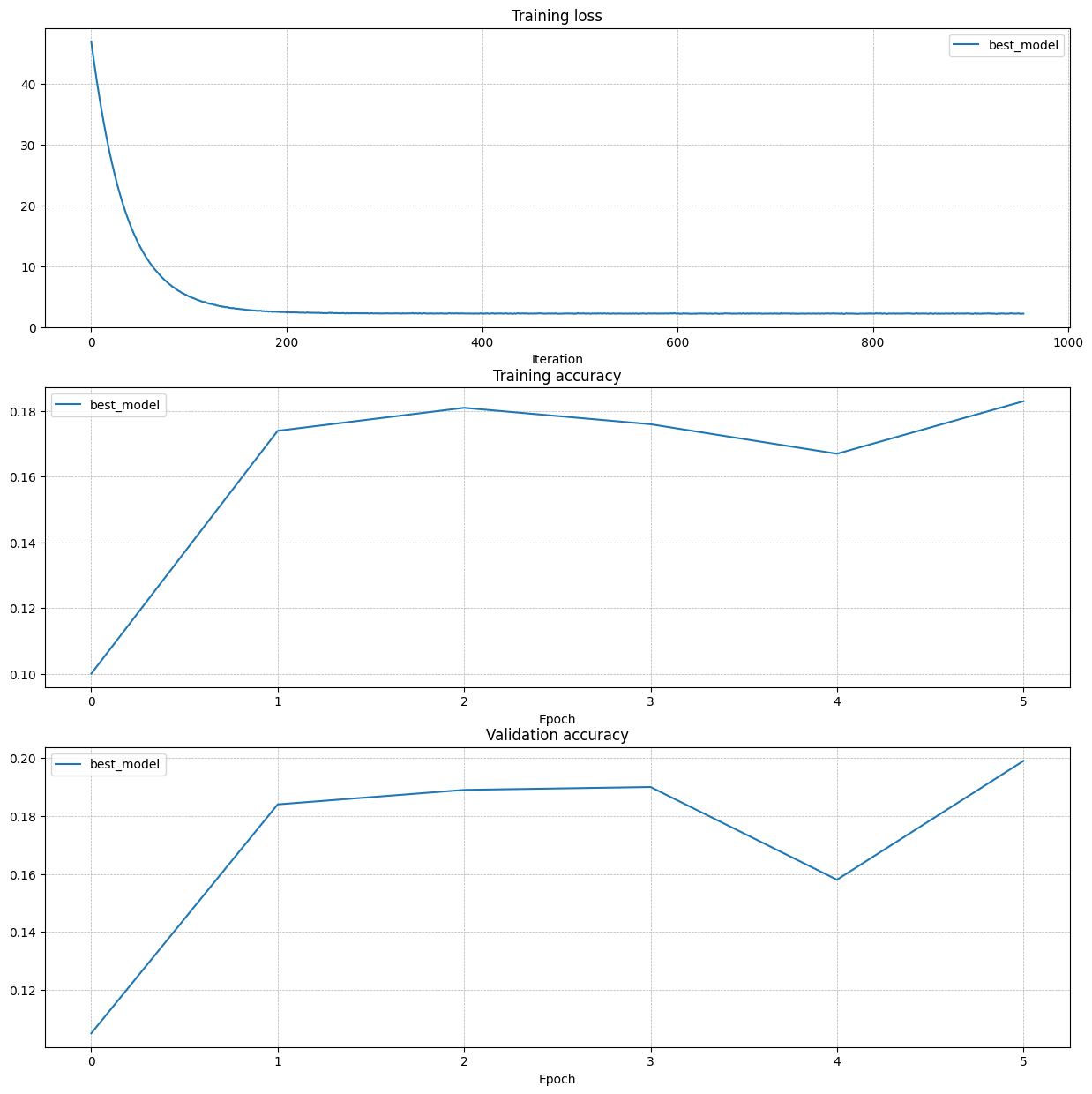
Train a Good Model!
Train the best fully connected model that you can on CIFAR-10, storing your best model in the best_model variable. We require you to get at least 50% accuracy on the validation set using a fully connected network.
If you are careful it should be possible to get accuracies above 55%, but we don’t require it for this part and won’t assign extra credit for doing so. Later in the assignment we will ask you to train the best convolutional network that you can on CIFAR-10, and we would prefer that you spend your effort working on convolutional networks rather than fully connected networks.
Note: You might find it useful to complete the BatchNormalization.ipynb and Dropout.ipynb notebooks before completing this part, since those techniques can help you train powerful models.
import itertools
best_model =None################################################################################# TODO: Train the best FullyConnectedNet that you can on CIFAR-10. You might ## find batch/layer normalization and dropout useful. Store your best model in ## the best_model variable. ################################################################################## *****START OF YOUR CODE (DO NOT DELETE/MODIFY THIS LINE)*****best_acc =-1best_solver =None#hidden_dims = [[100, 100, 100], [100,100,100,100]]hidden_dims = [[85, 85, 80, 80]]learning_rates = np.logspace(-3.8, -2.8, 8)weight_scales = np.logspace(-2, -1.6, 4)params =list(itertools.product(hidden_dims, learning_rates, weight_scales))for hd, lr, ws in params: model = FullyConnectedNet( hidden_dims=hd, input_dim =3*32*32, num_classes=10, normalization=None, reg=0.5, weight_scale=ws, ) solver = Solver( model=model, data=small_data, update_rule='adam', num_epochs=5, batch_size=256, optim_config={'learning_rate': lr}, verbose=False ) solver.train()if solver.best_val_acc > best_acc: best_model = model best_solver = solver best_acc = solver.best_val_acc best_lr, best_ws, best_hd = (lr, ws, hd)print('best valid acc yet: {} lr: {} ws: {} hd: {}'.format(best_acc, lr, ws, hd))fig, axes = plt.subplots(3, 1, figsize=(15, 15))axes[0].set_title('Training loss')axes[0].set_xlabel('Iteration')axes[1].set_title('Training accuracy')axes[1].set_xlabel('Epoch')axes[2].set_title('Validation accuracy')axes[2].set_xlabel('Epoch')axes[0].plot(best_solver.loss_history, label="best_model")axes[1].plot(best_solver.train_acc_history, label="best_model")axes[2].plot(best_solver.val_acc_history, label="best_model")for ax in axes: ax.legend(loc='best', ncol=4) ax.grid(linestyle='--', linewidth=0.5)plt.show()# *****END OF YOUR CODE (DO NOT DELETE/MODIFY THIS LINE)*****################################################################################# END OF YOUR CODE #################################################################################