# Setup cell.
import numpy as np
import matplotlib.pyplot as plt
from cs231n.classifiers.cnn import *
from cs231n.data_utils import get_CIFAR10_data
from cs231n.gradient_check import eval_numerical_gradient_array, eval_numerical_gradient
from cs231n.layers import *
from cs231n.fast_layers import *
from cs231n.solver import Solver

%matplotlib inline
plt.rcParams['figure.figsize'] = (10.0, 8.0) # set default size of plots
plt.rcParams['image.interpolation'] = 'nearest'
plt.rcParams['image.cmap'] = 'gray'

# for auto-reloading external modules
# see http://stackoverflow.com/questions/1907993/autoreload-of-modules-in-ipython
%load_ext autoreload
%autoreload 2

def rel_error(x, y):
  """ returns relative error """
return np.max(np.abs(x - y) / (np.maximum(1e-8, np.abs(x) + np.abs(y))))CS231N
This course is a deep dive into the details of deep learning architectures with a focus on learning end-to-end models for these tasks, particularly image classification
This page contains my solutions and approaches for the assignment All source codes of my solutions are available on GitHub
Convolutional Networks
So far we have worked with deep fully connected networks, using them to explore different optimization strategies and network architectures. Fully connected networks are a good testbed for experimentation because they are very computationally efficient, but in practice all state-of-the-art results use convolutional networks instead.
First you will implement several layer types that are used in convolutional networks. You will then use these layers to train a convolutional network on the CIFAR-10 dataset.
# Load the (preprocessed) CIFAR-10 data.
data = get_CIFAR10_data()
for k, v in list(data.items()):
    print(f"{k}: {v.shape}")
X_train: (49000, 3, 32, 32)
y_train: (49000,)
X_val: (1000, 3, 32, 32)
y_val: (1000,)
X_test: (1000, 3, 32, 32)
y_test: (1000,)Convolution: Naive Forward Pass
The core of a convolutional network is the convolution operation. In the file cs231n/layers.py, implement the forward pass for the convolution layer in the function conv_forward_naive.
You don’t have to worry too much about efficiency at this point; just write the code in whatever way you find most clear.
You can test your implementation by running the following:
def conv_forward_naive(x, w, b, conv_param):
    """
    A naive implementation of the forward pass for a convolutional layer.

    The input consists of N data points, each with C channels, height H and
    width W. We convolve each input with F different filters, where each filter
    spans all C channels and has height HH and width WW.

    Input:
    - x: Input data of shape (N, C, H, W)
    - w: Filter weights of shape (F, C, HH, WW)
    - b: Biases, of shape (F,)
    - conv_param: A dictionary with the following keys:
      - 'stride': The number of pixels between adjacent receptive fields in the
        horizontal and vertical directions.
      - 'pad': The number of pixels that will be used to zero-pad the input.


    During padding, 'pad' zeros should be placed symmetrically (i.e equally on both sides)
    along the height and width axes of the input. Be careful not to modfiy the original
    input x directly.

    Returns a tuple of:
    - out: Output data, of shape (N, F, H', W') where H' and W' are given by
      H' = 1 + (H + 2 * pad - HH) / stride
      W' = 1 + (W + 2 * pad - WW) / stride
    - cache: (x, w, b, conv_param)
    """
    def array_patches(array, kernel_width, kernel_height, stride):
      _, array_height, array_width = array.shape
      for i, y in enumerate(range(0, array_height - kernel_height + 1, stride)):
          for j, x in enumerate(range(0, array_width - kernel_width + 1, stride)):
              patch = array[:, y:y+kernel_height, x:x+kernel_width]
              yield (patch, i, j)

    out = None
    ###########################################################################
    # TODO: Implement the convolutional forward pass.                         #
    # Hint: you can use the function np.pad for padding.                      #
    ###########################################################################
    # *****START OF YOUR CODE (DO NOT DELETE/MODIFY THIS LINE)*****


    pad  = conv_param['pad']
    stride = conv_param['stride']
    N, C, H, W = x.shape
    F, C, HH, WW = w.shape

    assert (H + 2 * pad - HH) % stride == 0
    assert (W + 2 * pad -WW) % stride == 0

    oH = int(1 + (H + 2 * pad - HH) / stride)
    oW = int(1 + (W + 2 * pad - WW) / stride)
    out = np.zeros((N, F, oH, oW))

    x_pad = np.pad(x, ((0,0), (0,0), (pad,pad), (pad,pad)), mode='constant')

    for n, x_i in enumerate(x_pad): # iterate over all train samples
      for f, (w_j, b_j) in enumerate(list(zip(w, b))): # iterate over all filters and corresponding biases
        w_j_flat = w_j.flatten()
        for patch, height_index, width_index in array_patches(x_i, WW, HH, stride):
          patch_flat = patch.flatten()
          res = np.dot(w_j_flat.T, patch_flat) + b_j
          out[n, f, height_index, width_index] = res

    # print('conv_forward')
    # print('\tx.shape', x.shape)
    # print('\tx_pad.shape', x_pad.shape)
    # print('\tw.shape', w.shape)
    # print('\tb.shape', b.shape)
    # print('\tout.shape', out.shape)

    # *****END OF YOUR CODE (DO NOT DELETE/MODIFY THIS LINE)*****
    ###########################################################################
    #                             END OF YOUR CODE                            #
    ###########################################################################
    cache = (x, w, b, conv_param)
    return out, cache
x_shape = (2, 3, 4, 4)
w_shape = (3, 3, 4, 4)
x = np.linspace(-0.1, 0.5, num=np.prod(x_shape)).reshape(x_shape)
w = np.linspace(-0.2, 0.3, num=np.prod(w_shape)).reshape(w_shape)
b = np.linspace(-0.1, 0.2, num=3)
conv_param = {'stride': 2, 'pad': 1}
out, _ = conv_forward_naive(x, w, b, conv_param)
correct_out = np.array([[[[-0.08759809, -0.10987781],
[-0.18387192, -0.2109216 ]],
[[ 0.21027089, 0.21661097],
[ 0.22847626, 0.23004637]],
[[ 0.50813986, 0.54309974],
[ 0.64082444, 0.67101435]]],
[[[-0.98053589, -1.03143541],
[-1.19128892, -1.24695841]],
[[ 0.69108355, 0.66880383],
[ 0.59480972, 0.56776003]],
[[ 2.36270298, 2.36904306],
[ 2.38090835, 2.38247847]]]])
# Compare your output to ours; difference should be around e-8
print('Testing conv_forward_naive')
print('difference: ', rel_error(out, correct_out))Testing conv_forward_naive
difference: 2.2121476417505994e-08Aside: Image Processing via Convolutions
As fun way to both check your implementation and gain a better understanding of the type of operation that convolutional layers can perform, we will set up an input containing two images and manually set up filters that perform common image processing operations (grayscale conversion and edge detection). The convolution forward pass will apply these operations to each of the input images. We can then visualize the results as a sanity check.
from imageio import imread
from PIL import Image

kitten = imread('cs231n/notebook_images/kitten.jpg')
puppy = imread('cs231n/notebook_images/puppy.jpg')
# kitten is wide, and puppy is already square
d = kitten.shape[1] - kitten.shape[0]
kitten_cropped = kitten[:, d//2:-d//2, :]

img_size = 200   # Make this smaller if it runs too slow
resized_puppy = np.array(Image.fromarray(puppy).resize((img_size, img_size)))
resized_kitten = np.array(Image.fromarray(kitten_cropped).resize((img_size, img_size)))
x = np.zeros((2, 3, img_size, img_size))
x[0, :, :, :] = resized_puppy.transpose((2, 0, 1))
x[1, :, :, :] = resized_kitten.transpose((2, 0, 1))

# Set up a convolutional weights holding 2 filters, each 3x3
w = np.zeros((2, 3, 3, 3))

# The first filter converts the image to grayscale.
# Set up the red, green, and blue channels of the filter.
w[0, 0, :, :] = [[0, 0, 0], [0, 0.3, 0], [0, 0, 0]]
w[0, 1, :, :] = [[0, 0, 0], [0, 0.6, 0], [0, 0, 0]]
w[0, 2, :, :] = [[0, 0, 0], [0, 0.1, 0], [0, 0, 0]]

# Second filter detects horizontal edges in the blue channel.
w[1, 2, :, :] = [[1, 2, 1], [0, 0, 0], [-1, -2, -1]]

# Vector of biases. We don't need any bias for the grayscale
# filter, but for the edge detection filter we want to add 128
# to each output so that nothing is negative.
b = np.array([0, 128])

# Compute the result of convolving each input in x with each filter in w,
# offsetting by b, and storing the results in out.
out, _ = conv_forward_naive(x, w, b, {'stride': 1, 'pad': 1})

def imshow_no_ax(img, normalize=True):
    """ Tiny helper to show images as uint8 and remove axis labels """
    if normalize:
        img_max, img_min = np.max(img), np.min(img)
        img = 255.0 * (img - img_min) / (img_max - img_min)
    plt.imshow(img.astype('uint8'))
    plt.gca().axis('off')

# Show the original images and the results of the conv operation
plt.subplot(2, 3, 1)
imshow_no_ax(puppy, normalize=False)
plt.title('Original image')
plt.subplot(2, 3, 2)
imshow_no_ax(out[0, 0])
plt.title('Grayscale')
plt.subplot(2, 3, 3)
imshow_no_ax(out[0, 1])
plt.title('Edges')
plt.subplot(2, 3, 4)
imshow_no_ax(kitten_cropped, normalize=False)
plt.subplot(2, 3, 5)
imshow_no_ax(out[1, 0])
plt.subplot(2, 3, 6)
imshow_no_ax(out[1, 1])
plt.show()
DeprecationWarning: Starting with ImageIO v3 the behavior of this function will switch to that of iio.v3.imread. To keep the current behavior (and make this warning disappear) use `import imageio.v2 as imageio` or call `imageio.v2.imread` directly.
kitten = imread('cs231n/notebook_images/kitten.jpg')
<ipython-input-5-7950733600c3>:5: DeprecationWarning: Starting with ImageIO v3 the behavior of this function will switch to that of iio.v3.imread. To keep the current behavior (and make this warning disappear) use `import imageio.v2 as imageio` or call `imageio.v2.imread` directly.
puppy = imread('cs231n/notebook_images/puppy.jpg')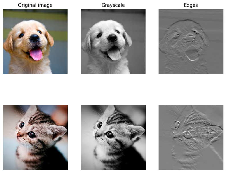
Convolution: Naive Backward Pass
Implement the backward pass for the convolution operation in the function conv_backward_naive in the file cs231n/layers.py. Again, you don’t need to worry too much about computational efficiency.
When you are done, run the following to check your backward pass with a numeric gradient check.
def conv_backward_naive(dout, cache):
    """
    A naive implementation of the backward pass for a convolutional layer.

    Inputs:
    - dout: Upstream derivatives.
    - cache: A tuple of (x, w, b, conv_param) as in conv_forward_naive

    Returns a tuple of:
    - dx: Gradient with respect to x
    - dw: Gradient with respect to w
    - db: Gradient with respect to b
    """
    dx, dw, db = None, None, None
    ###########################################################################
    # TODO: Implement the convolutional backward pass.                        #
    ###########################################################################
    # *****START OF YOUR CODE (DO NOT DELETE/MODIFY THIS LINE)*****

    # Generated with GPT-3

    x, w, b, conv_param = cache
    stride = conv_param['stride']
    pad = conv_param['pad']

    N, C, H, W = x.shape
    F, _, HH, WW = w.shape
    _, _, out_H, out_W = dout.shape

    dx = np.zeros_like(x)
    dw = np.zeros_like(w)
    db = np.zeros_like(b)

    x_pad = np.pad(x, ((0, 0), (0, 0), (pad, pad), (pad, pad)), mode='constant')

    dx_pad = np.pad(dx, ((0, 0), (0, 0), (pad, pad), (pad, pad)), mode='constant')

    for n in range(N):
        for f in range(F):
            for h_out in range(out_H):
                for w_out in range(out_W):
                    h_start = h_out * stride
                    h_end = h_start + HH
                    w_start = w_out * stride
                    w_end = w_start + WW

                    dx_pad[n, :, h_start:h_end, w_start:w_end] += w[f] * dout[n, f, h_out, w_out]
                    dw[f] += x_pad[n, :, h_start:h_end, w_start:w_end] * dout[n, f, h_out, w_out]
                    db[f] += dout[n, f, h_out, w_out]

    dx = dx_pad[:, :, pad:-pad, pad:-pad]

    # *****END OF YOUR CODE (DO NOT DELETE/MODIFY THIS LINE)*****
    ###########################################################################
    #                             END OF YOUR CODE                            #
    ###########################################################################
return dx, dw, dbnp.random.seed(231)
x = np.random.randn(4, 3, 5, 5)
w = np.random.randn(2, 3, 3, 3)
b = np.random.randn(2,)
dout = np.random.randn(4, 2, 5, 5)
conv_param = {'stride': 1, 'pad': 1}
dx_num = eval_numerical_gradient_array(lambda x: conv_forward_naive(x, w, b, conv_param)[0], x, dout)
dw_num = eval_numerical_gradient_array(lambda w: conv_forward_naive(x, w, b, conv_param)[0], w, dout)
db_num = eval_numerical_gradient_array(lambda b: conv_forward_naive(x, w, b, conv_param)[0], b, dout)
out, cache = conv_forward_naive(x, w, b, conv_param)
dx, dw, db = conv_backward_naive(dout, cache)
# Your errors should be around e-8 or less.
print('Testing conv_backward_naive function')
print('dx error: ', rel_error(dx, dx_num))
print('dw error: ', rel_error(dw, dw_num))
print('db error: ', rel_error(db, db_num))Testing conv_backward_naive function
dx error: 2.9516731319807213e-09
dw error: 5.185597891706744e-10
db error: 2.1494023503533904e-11Max-Pooling: Naive Forward Pass
Implement the forward pass for the max-pooling operation in the function max_pool_forward_naive in the file cs231n/layers.py. Again, don’t worry too much about computational efficiency.
Check your implementation by running the following:
def max_pool_forward_naive(x, pool_param):
    """
    A naive implementation of the forward pass for a max-pooling layer.

    Inputs:
    - x: Input data, of shape (N, C, H, W)
    - pool_param: dictionary with the following keys:
      - 'pool_height': The height of each pooling region
      - 'pool_width': The width of each pooling region
      - 'stride': The distance between adjacent pooling regions

    No padding is necessary here, eg you can assume:
      - (H - pool_height) % stride == 0
      - (W - pool_width) % stride == 0

    Returns a tuple of:
    - out: Output data, of shape (N, C, H', W') where H' and W' are given by
      H' = 1 + (H - pool_height) / stride
      W' = 1 + (W - pool_width) / stride
    - cache: (x, pool_param)
    """
    out = None
    ###########################################################################
    # TODO: Implement the max-pooling forward pass                            #
    ###########################################################################
    # *****START OF YOUR CODE (DO NOT DELETE/MODIFY THIS LINE)*****

    N, C, H, W = x.shape
    pool_height = pool_param['pool_height']
    pool_width = pool_param['pool_width']
    stride = pool_param['stride']

    out_H = int(1 + (H - pool_height) / stride)
    out_W = int(1 + (W - pool_width) / stride)

    out = np.zeros(((N, C, out_H, out_W)))

    for n in range(N):
        for c in range(C):
            for h_out in range(out_H):
                for w_out in range(out_W):
                    h_start = h_out * stride
                    h_end = h_start + pool_height
                    w_start = w_out * stride
                    w_end = w_start + pool_width

                    out[n, c, h_out, w_out] = x[n, c, h_start:h_end, w_start:w_end].max()


    # *****END OF YOUR CODE (DO NOT DELETE/MODIFY THIS LINE)*****
    ###########################################################################
    #                             END OF YOUR CODE                            #
    ###########################################################################
    cache = (x, pool_param)
    return out, cache
x_shape = (2, 3, 4, 4)
x = np.linspace(-0.3, 0.4, num=np.prod(x_shape)).reshape(x_shape)
pool_param = {'pool_width': 2, 'pool_height': 2, 'stride': 2}
out, _ = max_pool_forward_naive(x, pool_param)
correct_out = np.array([[[[-0.26315789, -0.24842105],
[-0.20421053, -0.18947368]],
[[-0.14526316, -0.13052632],
[-0.08631579, -0.07157895]],
[[-0.02736842, -0.01263158],
[ 0.03157895, 0.04631579]]],
[[[ 0.09052632, 0.10526316],
[ 0.14947368, 0.16421053]],
[[ 0.20842105, 0.22315789],
[ 0.26736842, 0.28210526]],
[[ 0.32631579, 0.34105263],
[ 0.38526316, 0.4 ]]]])
# Compare your output with ours. Difference should be on the order of e-8.
print('Testing max_pool_forward_naive function:')
print('difference: ', rel_error(out, correct_out))Testing max_pool_forward_naive function:
difference: 4.1666665157267834e-08Max-Pooling: Naive Backward
Implement the backward pass for the max-pooling operation in the function max_pool_backward_naive in the file cs231n/layers.py. You don’t need to worry about computational efficiency.
Check your implementation with numeric gradient checking by running the following:
def max_pool_backward_naive(dout, cache):
    """
    A naive implementation of the backward pass for a max-pooling layer.

    Inputs:
    - dout: Upstream derivatives
    - cache: A tuple of (x, pool_param) as in the forward pass.

    Returns:
    - dx: Gradient with respect to x
    """
    dx = None
    ###########################################################################
    # TODO: Implement the max-pooling backward pass                           #
    ###########################################################################
    # *****START OF YOUR CODE (DO NOT DELETE/MODIFY THIS LINE)*****

    x, pool_param = cache
    N, C, H, W = x.shape
    pool_height = pool_param['pool_height']
    pool_width = pool_param['pool_width']
    stride = pool_param['stride']

    out_H = int(1 + (H - pool_height) / stride)
    out_W = int(1 + (W - pool_width) / stride)

    dx = np.zeros(x.shape)

    for n in range(N):
        for c in range(C):
            for h_out in range(out_H):
                for w_out in range(out_W):
                    h_start = h_out * stride
                    h_end = h_start + pool_height
                    w_start = w_out * stride
                    w_end = w_start + pool_width

                    mask = x[n, c, h_start:h_end, w_start:w_end]
                    max_ind = np.unravel_index(np.argmax(mask, axis=None), mask.shape)
                    dx[n,c, h_start+max_ind[0], w_start+max_ind[1]] = dout[n,c,h_out,w_out]

    # *****END OF YOUR CODE (DO NOT DELETE/MODIFY THIS LINE)*****
    ###########################################################################
    #                             END OF YOUR CODE                            #
    ###########################################################################
return dxnp.random.seed(231)
x = np.random.randn(3, 2, 8, 8)
dout = np.random.randn(3, 2, 4, 4)
pool_param = {'pool_height': 2, 'pool_width': 2, 'stride': 2}
dx_num = eval_numerical_gradient_array(lambda x: max_pool_forward_naive(x, pool_param)[0], x, dout)
out, cache = max_pool_forward_naive(x, pool_param)
dx = max_pool_backward_naive(dout, cache)
# Your error should be on the order of e-12
print('Testing max_pool_backward_naive function:')
print('dx error: ', rel_error(dx, dx_num))Testing max_pool_backward_naive function:
dx error: 3.27562514223145e-12Fast Layers
Making convolution and pooling layers fast can be challenging. To spare you the pain, we’ve provided fast implementations of the forward and backward passes for convolution and pooling layers in the file cs231n/fast_layers.py.
The API for the fast versions of the convolution and pooling layers is exactly the same as the naive versions that you implemented above: the forward pass receives data, weights, and parameters and produces outputs and a cache object; the backward pass recieves upstream derivatives and the cache object and produces gradients with respect to the data and weights.
Note: The fast implementation for pooling will only perform optimally if the pooling regions are non-overlapping and tile the input. If these conditions are not met then the fast pooling implementation will not be much faster than the naive implementation.
You can compare the performance of the naive and fast versions of these layers by running the following:
# Rel errors should be around e-9 or less.
from cs231n.fast_layers import conv_forward_fast, conv_backward_fast
from time import time
np.random.seed(231)
x = np.random.randn(100, 3, 31, 31)
w = np.random.randn(25, 3, 3, 3)
b = np.random.randn(25,)
dout = np.random.randn(100, 25, 16, 16)
conv_param = {'stride': 2, 'pad': 1}

t0 = time()
out_naive, cache_naive = conv_forward_naive(x, w, b, conv_param)
t1 = time()
out_fast, cache_fast = conv_forward_fast(x, w, b, conv_param)
t2 = time()

print('Testing conv_forward_fast:')
print('Naive: %fs' % (t1 - t0))
print('Fast: %fs' % (t2 - t1))
print('Speedup: %fx' % ((t1 - t0) / (t2 - t1)))
print('Difference: ', rel_error(out_naive, out_fast))

t0 = time()
dx_naive, dw_naive, db_naive = conv_backward_naive(dout, cache_naive)
t1 = time()
dx_fast, dw_fast, db_fast = conv_backward_fast(dout, cache_fast)
t2 = time()

print('\nTesting conv_backward_fast:')
print('Naive: %fs' % (t1 - t0))
print('Fast: %fs' % (t2 - t1))
print('Speedup: %fx' % ((t1 - t0) / (t2 - t1)))
print('dx difference: ', rel_error(dx_naive, dx_fast))
print('dw difference: ', rel_error(dw_naive, dw_fast))
print('db difference: ', rel_error(db_naive, db_fast))
Testing conv_forward_fast:
Naive: 2.364269s
Fast: 0.010223s
Speedup: 231.260751x
Difference: 6.896970992227657e-11
Testing conv_backward_fast:
Naive: 10.624429s
Fast: 0.021898s
Speedup: 485.177349x
dx difference: 1.949764775345631e-11
dw difference: 3.681156828004736e-13
db difference: 3.481354613192702e-14# Relative errors should be close to 0.0.
from cs231n.fast_layers import max_pool_forward_fast, max_pool_backward_fast
np.random.seed(231)
x = np.random.randn(100, 3, 32, 32)
dout = np.random.randn(100, 3, 16, 16)
pool_param = {'pool_height': 2, 'pool_width': 2, 'stride': 2}
t0 = time()
out_naive, cache_naive = max_pool_forward_naive(x, pool_param)
t1 = time()
out_fast, cache_fast = max_pool_forward_fast(x, pool_param)
t2 = time()
print('Testing pool_forward_fast:')
print('Naive: %fs' % (t1 - t0))
print('fast: %fs' % (t2 - t1))
print('speedup: %fx' % ((t1 - t0) / (t2 - t1)))
print('difference: ', rel_error(out_naive, out_fast))
t0 = time()
dx_naive = max_pool_backward_naive(dout, cache_naive)
t1 = time()
dx_fast = max_pool_backward_fast(dout, cache_fast)
t2 = time()
print('\nTesting pool_backward_fast:')
print('Naive: %fs' % (t1 - t0))
print('fast: %fs' % (t2 - t1))
print('speedup: %fx' % ((t1 - t0) / (t2 - t1)))
print('dx difference: ', rel_error(dx_naive, dx_fast))Testing pool_forward_fast:
Naive: 0.216674s
fast: 0.006251s
speedup: 34.660374x
difference: 0.0
Testing pool_backward_fast:
Naive: 0.669985s
fast: 0.013189s
speedup: 50.799360x
dx difference: 0.0Convolutional “Sandwich” Layers
In the previous assignment, we introduced the concept of “sandwich” layers that combine multiple operations into commonly used patterns. In the file cs231n/layer_utils.py you will find sandwich layers that implement a few commonly used patterns for convolutional networks. Run the cells below to sanity check their usage.
from cs231n.layer_utils import conv_relu_pool_forward, conv_relu_pool_backward
np.random.seed(231)
x = np.random.randn(2, 3, 16, 16)
w = np.random.randn(3, 3, 3, 3)
b = np.random.randn(3,)
dout = np.random.randn(2, 3, 8, 8)
conv_param = {'stride': 1, 'pad': 1}
pool_param = {'pool_height': 2, 'pool_width': 2, 'stride': 2}

out, cache = conv_relu_pool_forward(x, w, b, conv_param, pool_param)
dx, dw, db = conv_relu_pool_backward(dout, cache)

dx_num = eval_numerical_gradient_array(lambda x: conv_relu_pool_forward(x, w, b, conv_param, pool_param)[0], x, dout)
dw_num = eval_numerical_gradient_array(lambda w: conv_relu_pool_forward(x, w, b, conv_param, pool_param)[0], w, dout)
db_num = eval_numerical_gradient_array(lambda b: conv_relu_pool_forward(x, w, b, conv_param, pool_param)[0], b, dout)

# Relative errors should be around e-8 or less
print('Testing conv_relu_pool')
print('dx error: ', rel_error(dx_num, dx))
print('dw error: ', rel_error(dw_num, dw))
print('db error: ', rel_error(db_num, db))
Testing conv_relu_pool
dx error: 9.591132621921372e-09
dw error: 5.802391137330214e-09
db error: 1.0146343411762047e-09from cs231n.layer_utils import conv_relu_forward, conv_relu_backward
np.random.seed(231)
x = np.random.randn(2, 3, 8, 8)
w = np.random.randn(3, 3, 3, 3)
b = np.random.randn(3,)
dout = np.random.randn(2, 3, 8, 8)
conv_param = {'stride': 1, 'pad': 1}
out, cache = conv_relu_forward(x, w, b, conv_param)
dx, dw, db = conv_relu_backward(dout, cache)
dx_num = eval_numerical_gradient_array(lambda x: conv_relu_forward(x, w, b, conv_param)[0], x, dout)
dw_num = eval_numerical_gradient_array(lambda w: conv_relu_forward(x, w, b, conv_param)[0], w, dout)
db_num = eval_numerical_gradient_array(lambda b: conv_relu_forward(x, w, b, conv_param)[0], b, dout)
# Relative errors should be around e-8 or less
print('Testing conv_relu:')
print('dx error: ', rel_error(dx_num, dx))
print('dw error: ', rel_error(dw_num, dw))
print('db error: ', rel_error(db_num, db))Testing conv_relu:
dx error: 1.5218619980349303e-09
dw error: 2.702022646099404e-10
db error: 1.451272393591721e-10Three-Layer Convolutional Network
Now that you have implemented all the necessary layers, we can put them together into a simple convolutional network.
Open the file cs231n/classifiers/cnn.py and complete the implementation of the ThreeLayerConvNet class. Remember you can use the fast/sandwich layers (already imported for you) in your implementation. Run the following cells to help you debug:
from builtins import object
import numpy as np

from ..layers import *
from ..fast_layers import *
from ..layer_utils import *


class ThreeLayerConvNet(object):
    """
    A three-layer convolutional network with the following architecture:

    conv - relu - 2x2 max pool - affine - relu - affine - softmax

    The network operates on minibatches of data that have shape (N, C, H, W)
    consisting of N images, each with height H and width W and with C input
    channels.
    """

    def __init__(
        self,
        input_dim=(3, 32, 32),
        num_filters=32,
        filter_size=7,
        hidden_dim=100,
        num_classes=10,
        weight_scale=1e-3,
        reg=0.0,
        dtype=np.float32,
    ):
        """
        Initialize a new network.

        Inputs:
        - input_dim: Tuple (C, H, W) giving size of input data
        - num_filters: Number of filters to use in the convolutional layer
        - filter_size: Width/height of filters to use in the convolutional layer
        - hidden_dim: Number of units to use in the fully-connected hidden layer
        - num_classes: Number of scores to produce from the final affine layer.
        - weight_scale: Scalar giving standard deviation for random initialization
          of weights.
        - reg: Scalar giving L2 regularization strength
        - dtype: numpy datatype to use for computation.
        """
        self.params = {}
        self.reg = reg
        self.dtype = dtype

        ############################################################################
        # TODO: Initialize weights and biases for the three-layer convolutional    #
        # network. Weights should be initialized from a Gaussian centered at 0.0   #
        # with standard deviation equal to weight_scale; biases should be          #
        # initialized to zero. All weights and biases should be stored in the      #
        #  dictionary self.params. Store weights and biases for the convolutional  #
        # layer using the keys 'W1' and 'b1'; use keys 'W2' and 'b2' for the       #
        # weights and biases of the hidden affine layer, and keys 'W3' and 'b3'    #
        # for the weights and biases of the output affine layer.                   #
        #                                                                          #
        # IMPORTANT: For this assignment, you can assume that the padding          #
        # and stride of the first convolutional layer are chosen so that           #
        # **the width and height of the input are preserved**. Take a look at      #
        # the start of the loss() function to see how that happens.                #
        ############################################################################
        # *****START OF YOUR CODE (DO NOT DELETE/MODIFY THIS LINE)*****


        #conv:
        """
          Input:
            - x: Input data of shape (N, C, H, W)
          Output:
            - out: Output data, of shape (N, F, H', W') where H' and W' are given by
              H' = 1 + (H + 2 * pad - HH) / stride
              W' = 1 + (W + 2 * pad - WW) / stride
        """
        #relu:
        """
          Input:
            - x: Inputs, of any shape
          Output:
            - out: Output, of the same shape as x
        """
        #max_pool:
        """
          Input:
            - x: Input data, of shape (N, C, H, W)
          Output:
            - out: Output data, of shape (N, C, H', W') where H' and W' are given by
              H' = 1 + (H - pool_height) / stride
              W' = 1 + (W - pool_width) / stride
        """
        # conv - relu -max_pool(2x2)
        """
          Input:
            - x: Input data of shape (N, C, H, W)
          Output:
            - out: (N, C, H', W') where H' and W' are given by
              H' = 1 + ( (1 + (H+2*pad - HH / stride)) - pool_height ) / stride
              W' = 1 + ( (1 + (W+2*pad - WW) / stride)) - pool_width ) / stride
        """

        C, H, W = input_dim

        # output shapes of 1st layer (conv-relu-pool)
          # conv_stride = 1
          # conv_pad = (filter_size - 1) // 2
          # pool_height = 2
          # pool_width = 2
          # pool_stride = 2
        o1H = 1 + (H - 2)//2 # 1 + ((1 + (H + 2*pad - HH) / stride_conv) - pool_height) / stride_pool
        o1W =  1 + (W - 2)//2 # 1 + ((1 + (H + 2 * pad - WW) / stride_conv) - pool_width) / stride_pool

        self.params['W1'] = np.random.normal(0.0, weight_scale, (num_filters, C, filter_size, filter_size))
        self.params['b1'] = np.zeros((num_filters, ))

        self.params['W2'] = np.random.normal(0.0, weight_scale, (num_filters*o1H*o1W, hidden_dim))
        self.params['b2'] = np.zeros((hidden_dim, ))

        self.params['W3'] = np.random.normal(0.0, weight_scale, (hidden_dim, num_classes))
        self.params['b3'] = np.zeros((num_classes, ))

        # *****END OF YOUR CODE (DO NOT DELETE/MODIFY THIS LINE)*****
        ############################################################################
        #                             END OF YOUR CODE                             #
        ############################################################################

        for k, v in self.params.items():
            self.params[k] = v.astype(dtype)

    def loss(self, X, y=None):
        """
        Evaluate loss and gradient for the three-layer convolutional network.

        Input / output: Same API as TwoLayerNet in fc_net.py.
        """
        W1, b1 = self.params["W1"], self.params["b1"]
        W2, b2 = self.params["W2"], self.params["b2"]
        W3, b3 = self.params["W3"], self.params["b3"]

        # pass conv_param to the forward pass for the convolutional layer
        # Padding and stride chosen to preserve the input spatial size
        filter_size = W1.shape[2]
        conv_param = {"stride": 1, "pad": (filter_size - 1) // 2}

        # pass pool_param to the forward pass for the max-pooling layer
        pool_param = {"pool_height": 2, "pool_width": 2, "stride": 2}

        scores = None
        ############################################################################
        # TODO: Implement the forward pass for the three-layer convolutional net,  #
        # computing the class scores for X and storing them in the scores          #
        # variable.                                                                #
        #                                                                          #
        # Remember you can use the functions defined in cs231n/fast_layers.py and  #
        # cs231n/layer_utils.py in your implementation (already imported).         #
        ############################################################################
        # *****START OF YOUR CODE (DO NOT DELETE/MODIFY THIS LINE)*****

        o1, c1 = conv_relu_pool_forward(X, W1, b1, conv_param, pool_param)
        o2, c2 = affine_relu_forward(o1, W2, b2)
        o3, c3 = affine_forward(o2, W3, b3)

        scores = o3

        # *****END OF YOUR CODE (DO NOT DELETE/MODIFY THIS LINE)*****
        ############################################################################
        #                             END OF YOUR CODE                             #
        ############################################################################

        if y is None:
            return scores

        loss, grads = 0, {}
        ############################################################################
        # TODO: Implement the backward pass for the three-layer convolutional net, #
        # storing the loss and gradients in the loss and grads variables. Compute  #
        # data loss using softmax, and make sure that grads[k] holds the gradients #
        # for self.params[k]. Don't forget to add L2 regularization!               #
        #                                                                          #
        # NOTE: To ensure that your implementation matches ours and you pass the   #
        # automated tests, make sure that your L2 regularization includes a factor #
        # of 0.5 to simplify the expression for the gradient.                      #
        ############################################################################
        # *****START OF YOUR CODE (DO NOT DELETE/MODIFY THIS LINE)*****

        loss, dout = softmax_loss(scores, y)
        do2, dw3, db3 = affine_backward(dout, c3)
        do1, dw2, db2 = affine_relu_backward(do2, c2)
        dX, dw1, db1 = conv_relu_pool_backward(do1, c1)

        loss += 0.5 * self.reg * ( np.sum(W1 * W1) + np.sum(W2 * W2) + np.sum(W3 * W3) )

        grads['W1'] = dw1 + (self.reg * W1)
        grads['W2'] = dw2 + (self.reg * W2)
        grads['W3'] = dw3 + (self.reg * W3)
        grads['b1'] = db1
        grads['b2'] = db2
        grads['b3'] = db3

        # *****END OF YOUR CODE (DO NOT DELETE/MODIFY THIS LINE)*****
        ############################################################################
        #                             END OF YOUR CODE                             #
        ############################################################################

        return loss, grads
Sanity Check Loss
After you build a new network, one of the first things you should do is sanity check the loss. When we use the softmax loss, we expect the loss for random weights (and no regularization) to be about log(C) for C classes. When we add regularization the loss should go up slightly.
model = ThreeLayerConvNet()

N = 50
X = np.random.randn(N, 3, 32, 32)
y = np.random.randint(10, size=N)

loss, grads = model.loss(X, y)
print('Initial loss (no regularization): ', loss)

model.reg = 0.5
loss, grads = model.loss(X, y)
print('Initial loss (with regularization): ', loss)
Initial loss (no regularization): 2.3025851358028335
Initial loss (with regularization): 2.508403341874687Gradient Check
After the loss looks reasonable, use numeric gradient checking to make sure that your backward pass is correct. When you use numeric gradient checking you should use a small amount of artifical data and a small number of neurons at each layer. Note: correct implementations may still have relative errors up to the order of e-2.
num_inputs = 2
input_dim = (3, 16, 16)
reg = 0.0
num_classes = 10
np.random.seed(231)
X = np.random.randn(num_inputs, *input_dim)
y = np.random.randint(num_classes, size=num_inputs)

model = ThreeLayerConvNet(
    num_filters=3,
    filter_size=3,
    input_dim=input_dim,
    hidden_dim=7,
    dtype=np.float64
)
loss, grads = model.loss(X, y)
# Errors should be small, but correct implementations may have
# relative errors up to the order of e-2
for param_name in sorted(grads):
    f = lambda _: model.loss(X, y)[0]
    param_grad_num = eval_numerical_gradient(f, model.params[param_name], verbose=False, h=1e-6)
    e = rel_error(param_grad_num, grads[param_name])
    print('%s max relative error: %e' % (param_name, rel_error(param_grad_num, grads[param_name])))
W1 max relative error: 3.053954e-04
W2 max relative error: 1.822722e-02
W3 max relative error: 3.063999e-04
b1 max relative error: 3.394850e-06
b2 max relative error: 2.516361e-03
b3 max relative error: 1.123715e-08Overfit Small Data
A nice trick is to train your model with just a few training samples. You should be able to overfit small datasets, which will result in very high training accuracy and comparatively low validation accuracy.
np.random.seed(231)

num_train = 100
small_data = {
  'X_train': data['X_train'][:num_train],
  'y_train': data['y_train'][:num_train],
  'X_val': data['X_val'],
  'y_val': data['y_val'],
}

model = ThreeLayerConvNet(weight_scale=1e-2)

solver = Solver(
    model,
    small_data,
    num_epochs=15,
    batch_size=50,
    update_rule='adam',
    optim_config={'learning_rate': 1e-3,},
    verbose=True,
    print_every=1
)
solver.train()
(Iteration 1 / 30) loss: 2.414060
(Epoch 0 / 15) train acc: 0.200000; val_acc: 0.137000
(Iteration 2 / 30) loss: 3.102925
(Epoch 1 / 15) train acc: 0.140000; val_acc: 0.087000
(Iteration 3 / 30) loss: 2.270330
(Iteration 4 / 30) loss: 2.096705
(Epoch 2 / 15) train acc: 0.240000; val_acc: 0.094000
(Iteration 5 / 30) loss: 1.838880
(Iteration 6 / 30) loss: 1.934188
(Epoch 3 / 15) train acc: 0.510000; val_acc: 0.173000
(Iteration 7 / 30) loss: 1.827912
(Iteration 8 / 30) loss: 1.639574
(Epoch 4 / 15) train acc: 0.520000; val_acc: 0.188000
(Iteration 9 / 30) loss: 1.330082
(Iteration 10 / 30) loss: 1.756115
(Epoch 5 / 15) train acc: 0.630000; val_acc: 0.167000
(Iteration 11 / 30) loss: 1.024162
(Iteration 12 / 30) loss: 1.041826
(Epoch 6 / 15) train acc: 0.750000; val_acc: 0.229000
(Iteration 13 / 30) loss: 1.142777
(Iteration 14 / 30) loss: 0.835706
(Epoch 7 / 15) train acc: 0.790000; val_acc: 0.247000
(Iteration 15 / 30) loss: 0.587786
(Iteration 16 / 30) loss: 0.645509
(Epoch 8 / 15) train acc: 0.820000; val_acc: 0.252000
(Iteration 17 / 30) loss: 0.786844
(Iteration 18 / 30) loss: 0.467054
(Epoch 9 / 15) train acc: 0.820000; val_acc: 0.178000
(Iteration 19 / 30) loss: 0.429880
(Iteration 20 / 30) loss: 0.635498
(Epoch 10 / 15) train acc: 0.900000; val_acc: 0.206000
(Iteration 21 / 30) loss: 0.365807
(Iteration 22 / 30) loss: 0.284220
(Epoch 11 / 15) train acc: 0.820000; val_acc: 0.201000
(Iteration 23 / 30) loss: 0.469343
(Iteration 24 / 30) loss: 0.509369
(Epoch 12 / 15) train acc: 0.920000; val_acc: 0.211000
(Iteration 25 / 30) loss: 0.111638
(Iteration 26 / 30) loss: 0.145388
(Epoch 13 / 15) train acc: 0.930000; val_acc: 0.213000
(Iteration 27 / 30) loss: 0.155575
(Iteration 28 / 30) loss: 0.143398
(Epoch 14 / 15) train acc: 0.960000; val_acc: 0.212000
(Iteration 29 / 30) loss: 0.158160
(Iteration 30 / 30) loss: 0.118934
(Epoch 15 / 15) train acc: 0.990000; val_acc: 0.220000# Print final training accuracy.
print(
"Small data training accuracy:",
solver.check_accuracy(small_data['X_train'], small_data['y_train'])
)Small data training accuracy: 0.82# Print final validation accuracy.
print(
"Small data validation accuracy:",
solver.check_accuracy(small_data['X_val'], small_data['y_val'])
)Small data validation accuracy: 0.252Plotting the loss, training accuracy, and validation accuracy should show clear overfitting:
plt.subplot(2, 1, 1)
plt.plot(solver.loss_history, 'o')
plt.xlabel('iteration')
plt.ylabel('loss')

plt.subplot(2, 1, 2)
plt.plot(solver.train_acc_history, '-o')
plt.plot(solver.val_acc_history, '-o')
plt.legend(['train', 'val'], loc='upper left')
plt.xlabel('epoch')
plt.ylabel('accuracy')
plt.show()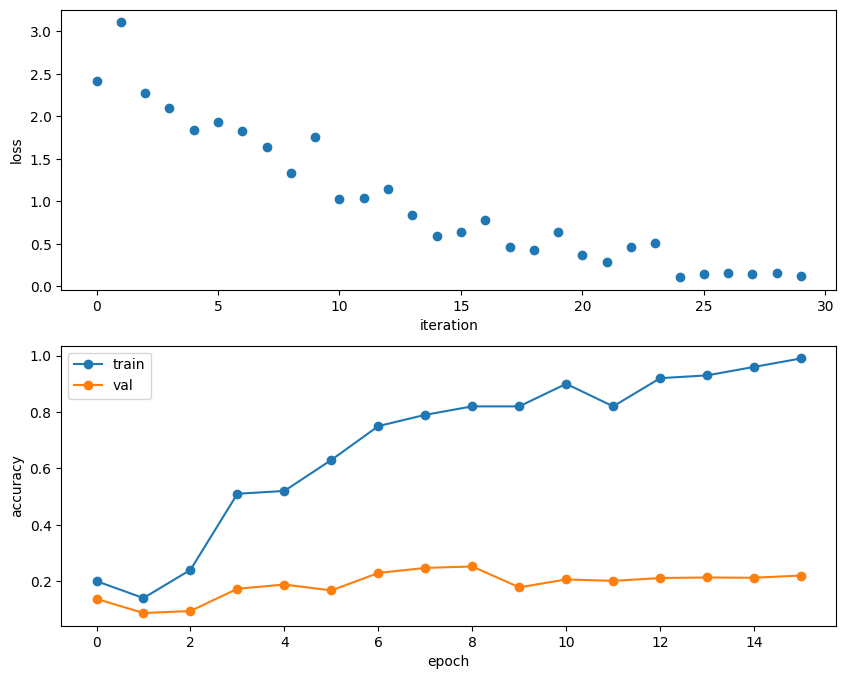
Train the Network
By training the three-layer convolutional network for one epoch, you should achieve greater than 40% accuracy on the training set:
model = ThreeLayerConvNet(weight_scale=0.001, hidden_dim=500, reg=0.001)

solver = Solver(
    model,
    data,
    num_epochs=1,
    batch_size=50,
    update_rule='adam',
    optim_config={'learning_rate': 1e-3,},
    verbose=True,
    print_every=20
)
solver.train()
(Iteration 1 / 980) loss: 2.304740
(Epoch 0 / 1) train acc: 0.103000; val_acc: 0.107000
(Iteration 21 / 980) loss: 2.098229
(Iteration 41 / 980) loss: 1.949734
(Iteration 61 / 980) loss: 1.823545
(Iteration 81 / 980) loss: 1.838017
(Iteration 101 / 980) loss: 1.876963
(Iteration 121 / 980) loss: 1.755037
(Iteration 141 / 980) loss: 1.914156
(Iteration 161 / 980) loss: 1.962187
(Iteration 181 / 980) loss: 1.743937
(Iteration 201 / 980) loss: 1.904272
(Iteration 221 / 980) loss: 1.856076
(Iteration 241 / 980) loss: 1.626667
(Iteration 261 / 980) loss: 1.556157
(Iteration 281 / 980) loss: 1.714100
(Iteration 301 / 980) loss: 1.697516
(Iteration 321 / 980) loss: 1.847386
(Iteration 341 / 980) loss: 1.699832
(Iteration 361 / 980) loss: 1.812523
(Iteration 381 / 980) loss: 1.426714
(Iteration 401 / 980) loss: 1.871958
(Iteration 421 / 980) loss: 1.601182
(Iteration 441 / 980) loss: 1.735095
(Iteration 461 / 980) loss: 1.913160
(Iteration 481 / 980) loss: 1.545488
(Iteration 501 / 980) loss: 1.581093
(Iteration 521 / 980) loss: 1.928734
(Iteration 541 / 980) loss: 1.686451
(Iteration 561 / 980) loss: 1.663179
(Iteration 581 / 980) loss: 1.450441
(Iteration 601 / 980) loss: 1.496559
(Iteration 621 / 980) loss: 1.531902
(Iteration 641 / 980) loss: 1.781726
(Iteration 661 / 980) loss: 1.723385
(Iteration 681 / 980) loss: 1.703042
(Iteration 701 / 980) loss: 1.531446
(Iteration 721 / 980) loss: 1.655756
(Iteration 741 / 980) loss: 1.653089
(Iteration 761 / 980) loss: 1.711886
(Iteration 781 / 980) loss: 1.931895
(Iteration 801 / 980) loss: 1.851152
(Iteration 821 / 980) loss: 1.659658
(Iteration 841 / 980) loss: 1.481572
(Iteration 861 / 980) loss: 1.796047
(Iteration 881 / 980) loss: 1.472391
(Iteration 901 / 980) loss: 1.580900
(Iteration 921 / 980) loss: 1.706728
(Iteration 941 / 980) loss: 1.685249
(Iteration 961 / 980) loss: 1.681575
(Epoch 1 / 1) train acc: 0.439000; val_acc: 0.451000# Print final training accuracy.
print(
"Full data training accuracy:",
solver.check_accuracy(data['X_train'], data['y_train'])
)Full data training accuracy: 0.44673469387755105# Print final validation accuracy.
print(
"Full data validation accuracy:",
solver.check_accuracy(data['X_val'], data['y_val'])
)Full data validation accuracy: 0.451Visualize Filters
You can visualize the first-layer convolutional filters from the trained network by running the following:
from cs231n.vis_utils import visualize_grid

grid = visualize_grid(model.params['W1'].transpose(0, 2, 3, 1))
plt.imshow(grid.astype('uint8'))
plt.axis('off')
plt.gcf().set_size_inches(5, 5)
plt.show()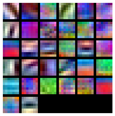
Spatial Batch Normalization
We already saw that batch normalization is a very useful technique for training deep fully connected networks. As proposed in the original paper (link in BatchNormalization.ipynb), batch normalization can also be used for convolutional networks, but we need to tweak it a bit; the modification will be called “spatial batch normalization.”
Normally, batch-normalization accepts inputs of shape (N, D) and produces outputs of shape (N, D), where we normalize across the minibatch dimension N. For data coming from convolutional layers, batch normalization needs to accept inputs of shape (N, C, H, W) and produce outputs of shape (N, C, H, W) where the N dimension gives the minibatch size and the (H, W) dimensions give the spatial size of the feature map.
If the feature map was produced using convolutions, then we expect every feature channel’s statistics e.g. mean, variance to be relatively consistent both between different images, and different locations within the same image – after all, every feature channel is produced by the same convolutional filter! Therefore, spatial batch normalization computes a mean and variance for each of the C feature channels by computing statistics over the minibatch dimension N as well the spatial dimensions H and W.
Spatial Batch Normalization: Forward Pass
In the file cs231n/layers.py, implement the forward pass for spatial batch normalization in the function spatial_batchnorm_forward. Check your implementation by running the following:
def spatial_batchnorm_forward(x, gamma, beta, bn_param):
    """
    Computes the forward pass for spatial batch normalization.

    Inputs:
    - x: Input data of shape (N, C, H, W)
    - gamma: Scale parameter, of shape (C,)
    - beta: Shift parameter, of shape (C,)
    - bn_param: Dictionary with the following keys:
      - mode: 'train' or 'test'; required
      - eps: Constant for numeric stability
      - momentum: Constant for running mean / variance. momentum=0 means that
        old information is discarded completely at every time step, while
        momentum=1 means that new information is never incorporated. The
        default of momentum=0.9 should work well in most situations.
      - running_mean: Array of shape (D,) giving running mean of features
      - running_var Array of shape (D,) giving running variance of features

    Returns a tuple of:
    - out: Output data, of shape (N, C, H, W)
    - cache: Values needed for the backward pass
    """
    out, cache = None, None

    ###########################################################################
    # TODO: Implement the forward pass for spatial batch normalization.       #
    #                                                                         #
    # HINT: You can implement spatial batch normalization by calling the      #
    # vanilla version of batch normalization you implemented above.           #
    # Your implementation should be very short; ours is less than five lines. #
    ###########################################################################
    # *****START OF YOUR CODE (DO NOT DELETE/MODIFY THIS LINE)*****

    N, C, H, W = x.shape
    x_ = x.transpose(0,2,3,1).reshape(N*H*W, C)
    out_, cache = batchnorm_forward(x_, gamma, beta, bn_param)
    out = out_.reshape(N, H, W, C).transpose(0,3,1,2)

    # *****END OF YOUR CODE (DO NOT DELETE/MODIFY THIS LINE)*****
    ###########################################################################
    #                             END OF YOUR CODE                            #
    ###########################################################################

return out, cachenp.random.seed(231)
# Check the training-time forward pass by checking means and variances
# of features both before and after spatial batch normalization.
N, C, H, W = 2, 3, 4, 5
x = 4 * np.random.randn(N, C, H, W) + 10
print('Before spatial batch normalization:')
print(' shape: ', x.shape)
print(' means: ', x.mean(axis=(0, 2, 3)))
print(' stds: ', x.std(axis=(0, 2, 3)))
# Means should be close to zero and stds close to one
gamma, beta = np.ones(C), np.zeros(C)
bn_param = {'mode': 'train'}
out, _ = spatial_batchnorm_forward(x, gamma, beta, bn_param)
print('After spatial batch normalization:')
print(' shape: ', out.shape)
print(' means: ', out.mean(axis=(0, 2, 3)))
print(' stds: ', out.std(axis=(0, 2, 3)))
# Means should be close to beta and stds close to gamma
gamma, beta = np.asarray([3, 4, 5]), np.asarray([6, 7, 8])
out, _ = spatial_batchnorm_forward(x, gamma, beta, bn_param)
print('After spatial batch normalization (nontrivial gamma, beta):')
print(' shape: ', out.shape)
print(' means: ', out.mean(axis=(0, 2, 3)))
print(' stds: ', out.std(axis=(0, 2, 3)))Before spatial batch normalization:
shape: (2, 3, 4, 5)
means: [9.33463814 8.90909116 9.11056338]
stds: [3.61447857 3.19347686 3.5168142 ]
After spatial batch normalization:
shape: (2, 3, 4, 5)
means: [ 5.85642645e-16 5.82867088e-17 -8.88178420e-17]
stds: [0.99999962 0.99999951 0.9999996 ]
After spatial batch normalization (nontrivial gamma, beta):
shape: (2, 3, 4, 5)
means: [6. 7. 8.]
stds: [2.99999885 3.99999804 4.99999798]np.random.seed(231)
# Check the test-time forward pass by running the training-time
# forward pass many times to warm up the running averages, and then
# checking the means and variances of activations after a test-time
# forward pass.
N, C, H, W = 10, 4, 11, 12
bn_param = {'mode': 'train'}
gamma = np.ones(C)
beta = np.zeros(C)
for t in range(50):
x = 2.3 * np.random.randn(N, C, H, W) + 13
spatial_batchnorm_forward(x, gamma, beta, bn_param)
bn_param['mode'] = 'test'
x = 2.3 * np.random.randn(N, C, H, W) + 13
a_norm, _ = spatial_batchnorm_forward(x, gamma, beta, bn_param)
# Means should be close to zero and stds close to one, but will be
# noisier than training-time forward passes.
print('After spatial batch normalization (test-time):')
print(' means: ', a_norm.mean(axis=(0, 2, 3)))
print(' stds: ', a_norm.std(axis=(0, 2, 3)))After spatial batch normalization (test-time):
means: [-0.08034406 0.07562881 0.05716371 0.04378383]
stds: [0.96718744 1.0299714 1.02887624 1.00585577]Spatial Batch Normalization: Backward Pass
In the file cs231n/layers.py, implement the backward pass for spatial batch normalization in the function spatial_batchnorm_backward. Run the following to check your implementation using a numeric gradient check:
def spatial_batchnorm_backward(dout, cache):
    """
    Computes the backward pass for spatial batch normalization.

    Inputs:
    - dout: Upstream derivatives, of shape (N, C, H, W)
    - cache: Values from the forward pass

    Returns a tuple of:
    - dx: Gradient with respect to inputs, of shape (N, C, H, W)
    - dgamma: Gradient with respect to scale parameter, of shape (C,)
    - dbeta: Gradient with respect to shift parameter, of shape (C,)
    """
    dx, dgamma, dbeta = None, None, None

    ###########################################################################
    # TODO: Implement the backward pass for spatial batch normalization.      #
    #                                                                         #
    # HINT: You can implement spatial batch normalization by calling the      #
    # vanilla version of batch normalization you implemented above.           #
    # Your implementation should be very short; ours is less than five lines. #
    ###########################################################################
    # *****START OF YOUR CODE (DO NOT DELETE/MODIFY THIS LINE)*****

    N, C, H, W = dout.shape
    dout_ = dout.transpose(0,2,3,1).reshape(N*H*W, C)
    dx_, dgamma, dbeta = batchnorm_backward_alt(dout_, cache)
    dx = dx_.reshape(N, H, W, C).transpose(0, 3, 1, 2)

    # *****END OF YOUR CODE (DO NOT DELETE/MODIFY THIS LINE)*****
    ###########################################################################
    #                             END OF YOUR CODE                            #
    ###########################################################################

return dx, dgamma, dbetanp.random.seed(231)
N, C, H, W = 2, 3, 4, 5
x = 5 * np.random.randn(N, C, H, W) + 12
gamma = np.random.randn(C)
beta = np.random.randn(C)
dout = np.random.randn(N, C, H, W)
bn_param = {'mode': 'train'}
fx = lambda x: spatial_batchnorm_forward(x, gamma, beta, bn_param)[0]
fg = lambda a: spatial_batchnorm_forward(x, gamma, beta, bn_param)[0]
fb = lambda b: spatial_batchnorm_forward(x, gamma, beta, bn_param)[0]
dx_num = eval_numerical_gradient_array(fx, x, dout)
da_num = eval_numerical_gradient_array(fg, gamma, dout)
db_num = eval_numerical_gradient_array(fb, beta, dout)
#You should expect errors of magnitudes between 1e-12~1e-06
_, cache = spatial_batchnorm_forward(x, gamma, beta, bn_param)
dx, dgamma, dbeta = spatial_batchnorm_backward(dout, cache)
print('dx error: ', rel_error(dx_num, dx))
print('dgamma error: ', rel_error(da_num, dgamma))
print('dbeta error: ', rel_error(db_num, dbeta))dx error: 3.0838468285639314e-07
dgamma error: 7.09738489671469e-12
dbeta error: 3.275608725278405e-12Spatial Group Normalization
In the previous notebook, we mentioned that Layer Normalization is an alternative normalization technique that mitigates the batch size limitations of Batch Normalization. However, as the authors of [2] observed, Layer Normalization does not perform as well as Batch Normalization when used with Convolutional Layers:
With fully connected layers, all the hidden units in a layer tend to make similar contributions to the final prediction, and re-centering and rescaling the summed inputs to a layer works well. However, the assumption of similar contributions is no longer true for convolutional neural networks. The large number of the hidden units whose receptive fields lie near the boundary of the image are rarely turned on and thus have very different statistics from the rest of the hidden units within the same layer.
The authors of [3] propose an intermediary technique. In contrast to Layer Normalization, where you normalize over the entire feature per-datapoint, they suggest a consistent splitting of each per-datapoint feature into G groups and a per-group per-datapoint normalization instead.
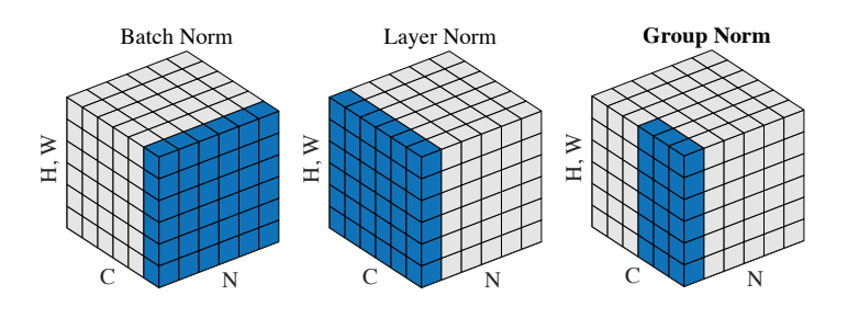
Even though an assumption of equal contribution is still being made within each group, the authors hypothesize that this is not as problematic, as innate grouping arises within features for visual recognition. One example they use to illustrate this is that many high-performance handcrafted features in traditional computer vision have terms that are explicitly grouped together. Take for example Histogram of Oriented Gradients [4] – after computing histograms per spatially local block, each per-block histogram is normalized before being concatenated together to form the final feature vector.
You will now implement Group Normalization.
[3] Wu, Yuxin, and Kaiming He. “Group Normalization.” arXiv preprint arXiv:1803.08494 (2018).
Spatial Group Normalization: Forward Pass
In the file cs231n/layers.py, implement the forward pass for group normalization in the function spatial_groupnorm_forward. Check your implementation by running the following:
def spatial_groupnorm_forward(x, gamma, beta, G, gn_param):
    """
    Computes the forward pass for spatial group normalization.
    In contrast to layer normalization, group normalization splits each entry
    in the data into G contiguous pieces, which it then normalizes independently.
    Per feature shifting and scaling are then applied to the data, in a manner identical to that of batch normalization and layer normalization.

    Inputs:
    - x: Input data of shape (N, C, H, W)
    - gamma: Scale parameter, of shape (1, C, 1, 1)
    - beta: Shift parameter, of shape (1, C, 1, 1)
    - G: Integer mumber of groups to split into, should be a divisor of C
    - gn_param: Dictionary with the following keys:
      - eps: Constant for numeric stability

    Returns a tuple of:
    - out: Output data, of shape (N, C, H, W)
    - cache: Values needed for the backward pass
    """
    out, cache = None, None
    eps = gn_param.get("eps", 1e-5)
    ###########################################################################
    # TODO: Implement the forward pass for spatial group normalization.       #
    # This will be extremely similar to the layer norm implementation.        #
    # In particular, think about how you could transform the matrix so that   #
    # the bulk of the code is similar to both train-time batch normalization  #
    # and layer normalization!                                                #
    ###########################################################################
    # *****START OF YOUR CODE (DO NOT DELETE/MODIFY THIS LINE)*****

    N, C, H, W = x.shape
    x = x.reshape(N, G, C // G, H, W)
    mu = np.mean(x, axis=(2,3,4), keepdims=True)
    # var = np.var(x, axis=(2,3,4), keepdims=True)

    xmu = x - mu
    sq = xmu**2
    var = 1./(C//G * H * W) * np.sum(sq, axis=(2,3,4), keepdims=True)
    sqrtvar = np.sqrt(var + eps)
    ivar = 1./ sqrtvar
    xhat = xmu * ivar
    xhat = xhat.reshape(N, C, H, W)
    gammax = gamma * xhat
    out = gammax + beta

    # x = (x - mean) / np.sqrt(var + eps)
    # x = x.reshape(N, C, H, W)
    # out = x * gamma + beta


    cache = (xhat,gamma,xmu,ivar,sqrtvar,var,eps,G, sq, mu, gammax)


    # *****END OF YOUR CODE (DO NOT DELETE/MODIFY THIS LINE)*****
    ###########################################################################
    #                             END OF YOUR CODE                            #
    ###########################################################################
return out, cachenp.random.seed(231)
# Check the training-time forward pass by checking means and variances
# of features both before and after spatial batch normalization.
N, C, H, W = 2, 6, 4, 5
G = 2
x = 4 * np.random.randn(N, C, H, W) + 10
x_g = x.reshape((N*G,-1))
print('Before spatial group normalization:')
print(' shape: ', x.shape)
print(' means: ', x_g.mean(axis=1))
print(' stds: ', x_g.std(axis=1))
# Means should be close to zero and stds close to one
gamma, beta = np.ones((1,C,1,1)), np.zeros((1,C,1,1))
bn_param = {'mode': 'train'}
out, _ = spatial_groupnorm_forward(x, gamma, beta, G, bn_param)
out_g = out.reshape((N*G,-1))
print('After spatial group normalization:')
print(' shape: ', out.shape)
print(' means: ', out_g.mean(axis=1))
print(' stds: ', out_g.std(axis=1))Before spatial group normalization:
shape: (2, 6, 4, 5)
means: [9.72505327 8.51114185 8.9147544 9.43448077]
stds: [3.67070958 3.09892597 4.27043622 3.97521327]
After spatial group normalization:
shape: (2, 6, 4, 5)
means: [-2.14643118e-16 5.25505565e-16 2.58126853e-16 -3.62672855e-16]
stds: [0.99999963 0.99999948 0.99999973 0.99999968]Spatial Group Normalization: Backward Pass
In the file cs231n/layers.py, implement the backward pass for spatial batch normalization in the function spatial_groupnorm_backward. Run the following to check your implementation using a numeric gradient check:
def spatial_groupnorm_backward(dout, cache):
    """
    Computes the backward pass for spatial group normalization.

    Inputs:
    - dout: Upstream derivatives, of shape (N, C, H, W)
    - cache: Values from the forward pass

    Returns a tuple of:
    - dx: Gradient with respect to inputs, of shape (N, C, H, W)
    - dgamma: Gradient with respect to scale parameter, of shape (1, C, 1, 1)
    - dbeta: Gradient with respect to shift parameter, of shape (1, C, 1, 1)
    """
    dx, dgamma, dbeta = None, None, None

    ###########################################################################
    # TODO: Implement the backward pass for spatial group normalization.      #
    # This will be extremely similar to the layer norm implementation.        #
    ###########################################################################
    # *****START OF YOUR CODE (DO NOT DELETE/MODIFY THIS LINE)*****

    #unpack the cache variables
    xhat,gamma,xmu,ivar,sqrtvar,var,eps,G, sq, mu, gammax = cache
    print('xhat.shape:', xhat.shape)
    print('gamma.shape:', gamma.shape)
    print('xmu.shape:', xmu.shape)
    print('ivar.shape:', ivar.shape)
    print('sqrtvar.shape:', sqrtvar.shape)
    print('var.shape:', var.shape)
    print('sq.shape:', sq.shape)
    print('mu.shape:', mu.shape)
    print('gammax.shape:', gammax.shape)
    print('dout.shape:', dout.shape)
    N,C,H,W = dout.shape

    #step9
    print('step-9 | begin')
    dbeta = 1 * np.sum(dout, axis=(0,2,3), keepdims=True)
    dgammax = dout
    print('\t dbeta.shape:', dbeta.shape)
    print('\t dgammax.shape:', dgammax.shape)

    #step8
    print('step-8 | begin')
    dgamma = np.sum(dgammax*xhat, axis=(0,2,3), keepdims=True)
    dxhat_ = dgammax * gamma
    dxhat = dxhat_.reshape(N, G, C // G, H, W)
    print('\t dgamma.shape:', dgamma.shape)
    print('\t dxhat_.shape:', dxhat_.shape)
    print('\t dxhat.shape:', dxhat.shape)

    #step7
    print('step-7 | begin')
    divar = np.sum(dxhat*xmu, axis=(2,3,4), keepdims=True)
    dxmu1 = dxhat * ivar
    print('\t dxmu1.shape:', dxmu1.shape)
    print('\t divar.shape:', divar.shape)

    #step6
    print('step-6 | begin')
    dsqrtvar = divar * (-1 / sqrtvar**2)
    print('\t dsqrtvar.shape:', dsqrtvar.shape)

    #step5
    print('step-5 | begin')
    dvar = 0.5 * (1 / np.sqrt(var + eps)) * dsqrtvar
    print('\t dvar.shape:', dvar.shape)

    #step4
    print('step-4 | begin')
    dsq = 1. /(C//G * H * W) * np.ones((N, G, C // G, H, W)) * dvar
    print('\t dsq.shape:', dsq.shape)

    #step3
    print('step-3 | begin')
    dxmu2 = 2 * xmu * dsq
    print('\t dxmu2.shape:', dxmu2.shape)

    #step2
    print('step-2 | begin')
    dx1 = (1 * (dxmu1 + dxmu2)).reshape(N, C, H, W)
    dmu = -1 * np.sum((dxmu1+dxmu2), axis=(2,3,4), keepdims=True)
    print('\t dx1.shape:', dx1.shape)
    print('\t dmu.shape:', dmu.shape)

    #step1
    print('step-1 | begin')
    dx2 = (1. / (C//G * H * W) * np.ones((N, G, C // G, H, W)) * dmu).reshape(N, C, H, W)
    print('\t dx2.shape:', dx2.shape)

    #step0
    print('step-0 | begin')
    dx = dx1 + dx2
    print('\t dx.shape:', dx.shape)

    # *****END OF YOUR CODE (DO NOT DELETE/MODIFY THIS LINE)*****
    ###########################################################################
    #                             END OF YOUR CODE                            #
    ###########################################################################
return dx, dgamma, dbetanp.random.seed(231)
N, C, H, W = 2, 6, 4, 5
G = 2
x = 5 * np.random.randn(N, C, H, W) + 12
gamma = np.random.randn(1,C,1,1)
beta = np.random.randn(1,C,1,1)
dout = np.random.randn(N, C, H, W)
gn_param = {}
fx = lambda x: spatial_groupnorm_forward(x, gamma, beta, G, gn_param)[0]
fg = lambda a: spatial_groupnorm_forward(x, gamma, beta, G, gn_param)[0]
fb = lambda b: spatial_groupnorm_forward(x, gamma, beta, G, gn_param)[0]
dx_num = eval_numerical_gradient_array(fx, x, dout)
da_num = eval_numerical_gradient_array(fg, gamma, dout)
db_num = eval_numerical_gradient_array(fb, beta, dout)
_, cache = spatial_groupnorm_forward(x, gamma, beta, G, gn_param)
dx, dgamma, dbeta = spatial_groupnorm_backward(dout, cache)
# You should expect errors of magnitudes between 1e-12 and 1e-07.
print('dx error: ', rel_error(dx_num, dx))
print('dgamma error: ', rel_error(da_num, dgamma))
print('dbeta error: ', rel_error(db_num, dbeta))xhat.shape: (2, 6, 4, 5)
gamma.shape: (1, 6, 1, 1)
xmu.shape: (2, 2, 3, 4, 5)
ivar.shape: (2, 2, 1, 1, 1)
sqrtvar.shape: (2, 2, 1, 1, 1)
var.shape: (2, 2, 1, 1, 1)
sq.shape: (2, 2, 3, 4, 5)
mu.shape: (2, 2, 1, 1, 1)
gammax.shape: (2, 6, 4, 5)
dout.shape: (2, 6, 4, 5)
step-9 | begin
dbeta.shape: (1, 6, 1, 1)
dgammax.shape: (2, 6, 4, 5)
step-8 | begin
dgamma.shape: (1, 6, 1, 1)
dxhat_.shape: (2, 6, 4, 5)
dxhat.shape: (2, 2, 3, 4, 5)
step-7 | begin
dxmu1.shape: (2, 2, 3, 4, 5)
divar.shape: (2, 2, 1, 1, 1)
step-6 | begin
dsqrtvar.shape: (2, 2, 1, 1, 1)
step-5 | begin
dvar.shape: (2, 2, 1, 1, 1)
step-4 | begin
dsq.shape: (2, 2, 3, 4, 5)
step-3 | begin
dxmu2.shape: (2, 2, 3, 4, 5)
step-2 | begin
dx1.shape: (2, 6, 4, 5)
dmu.shape: (2, 2, 1, 1, 1)
step-1 | begin
dx2.shape: (2, 6, 4, 5)
step-0 | begin
dx.shape: (2, 6, 4, 5)
dx error: 6.345904562232329e-08
dgamma error: 1.0546047434202244e-11
dbeta error: 3.810857316122484e-12